2. Conditional probability

2.1. Definition and intuition

When faced with new information, it is often necessary to adjust our beliefs or probabilities accordingly. This is where the concept of conditional probability comes into play. Conditional probability allows us to quantify the likelihood of an event \( A \), given that another event \( B \) has already occurred. It is defined mathematically as:

\[\begin{equation*} \mathbb{P}[A \mid B] = \frac{\mathbb{P}[A \cap B]}{\mathbb{P}[B]} \quad \text{for} \quad \mathbb{P}[B] > 0. \end{equation*}\]

In essence, this formula narrows the probability of \( A \) by focusing only on the outcomes in which \( B \) happens, as the following discussions illustrate.

Finite sample space: Visualizing outcomes. (This is Intuition 2.2.3 from [BH19].) The leftmost panel of Figure 2.1 illustrates a finite sample space where each possible outcome is represented as a pebble.

Fig. 2.1 Visualization of \(\mathbb{P}[A \mid B]\). This is Figure 2.1 from [BH19].

It also illustrates two events \(A\) and \(B\), which are sets of outcomes, i.e., sets of pebbles. Suppose we know that event \(B\) occurred, which means we can disregard all outcomes in \(B^c\), as in the middle panel of Figure 2.1. To compute \(\mathbb{P}[A \mid B]\) (the probability \(A\) occurs given that \(B\) occurred), we normalize the probabilities of the remaining outcomes to maintain a total probability of 1, as in the rightmost panel of Figure 2.1. This normalization explains the denominator of \(\mathbb{P}[A \mid B] = \frac{\mathbb{P}[A \cap B]}{\mathbb{P}[B]}\). If all outcomes are equally likely, then \(\mathbb{P}[A \mid B] = \frac{1}{4}\).

Rolling a die. Imagine rolling a die repeatedly, as in the following figure.

Fig. 2.2 Rolling a die. Rolls where the number is at least 4 are circled and rolls where the number is odd are underlined.

Suppose \( B \) is the event that the outcome is greater than or equal to 4 (marked by a circle in Figure 2.2), and \( A \) is the event that the outcome is odd (underlined). By observing the rolls where \( B \) occurs, we can estimate the probability that \( A \) also occurs. In the example above, the fraction of times \( A \) occurs when \( B \) happens is \(\frac{2}{6}\). This is a (frequentist) intuition that helps explain why \(\mathbb{P}[A \mid B] = \frac{1}{3}\).

Example: Bears vs. Packers.

This example is from [Sev20].

We can generalize the coin-flipping example to more practical “experiments”, such as football games where the Bears play the Packers at home. For intuition, as in the coin-flipping example, we can interpret the probability of an event as the long-run relative frequency of the event happening over a long sequence of games. Let \( A \) be the event that the Bears win. If, over this long sequence of games, \(A\) occurs about 25% of the time, we can interpret this as meaning that \( \mathbb{P}[A] = 0.25 \). Let \(B\) be the event that the Bears’ quarterback throws four interceptions during the at-home game. Suppose that, in our long sequence of games in which the Bears’ quarterback throws an interception (i.e., \(B\) occurs), the Bears win about 5% of the time. This would mean that the conditional probability of the Bears winning, given that their quarterback throws four interceptions, drops to \( \mathbb{P}[A \mid B] = 0.05 \): the interceptions negatively affect their chances of winning.

Example: Tossing coins.

Suppose we toss a coin twice. We will explore conditional probability through two scenarios: Question: What is the probability that both flips land on heads, given that the first flip lands on heads?

The sample space is \( S = \{(H,H), (H,T), (T,H), (T,T)\} \). The event that both flips land on heads is \( A = \{(H,H)\} \), and the event that the first flip lands on heads is \( B = \{(H,H), (H,T)\} \). Therefore, \(\mathbb{P}[B] = \frac{1}{2}\) and \(\mathbb{P}[A \cap B] = \frac{|\{HH\}|}{|S|} = \frac{1}{4}\). Therefore,

\[\begin{equation*} \mathbb{P}[A \mid B] = \frac{\mathbb{P}[A \cap B]}{\mathbb{P}[B]} = \frac{1/4}{1/2} = \frac{1}{2}. \end{equation*}\]

Question: What is the probability that both flips land on heads, given that at least one flip lands on heads?

The event that at least one flip lands on heads is \( C = \{(H,H), (H,T), (T,H)\} \). The conditional probability is:

\[\begin{equation*} \mathbb{P}[A \mid C] = \frac{\mathbb{P}[A \cap C]}{\mathbb{P}[C]} = \frac{1/4}{3/4} = \frac{1}{3}. \end{equation*}\]

It is important to keep in mind that conditional probabilities still obey the basic rules of probability. For example, \( \mathbb{P}[A \mid B] = 1 - \mathbb{P}[A^c \mid B] \). This means that if the probability of the Bears winning after their quarterback throws four interceptions is \( 0.05 \), the probability of them not winning given the same information is \( 0.95 \).

2.2. Bayes’ rule and the law of total probability

In this section, we will cover two famous tools for calculating conditional probabilities: Bayes’ rule and the law of total probability.

Bayes’ rule.

Bayes’ rule tells us that

\[\begin{equation*} \mathbb{P}[A \mid B] = \frac{\mathbb{P}[B \mid A] \mathbb{P}[A]}{\mathbb{P}[B]}. \end{equation*}\]

This fact follows simply from the observation that

1. \(\mathbb{P}[A \mid B] = \frac{\mathbb{P}[A \cap B]}{\mathbb{P}[B]}\), which means that \(\mathbb{P}[A \cap B] = \mathbb{P}[A \mid B]\mathbb{P}[B]\).

2. Moreover, \(\mathbb{P}[B \mid A] = \frac{\mathbb{P}[A \cap B]}{\mathbb{P}[A]}\), which means that \(\mathbb{P}[A \cap B] = \mathbb{P}[B \mid A]\mathbb{P}[A]\).

As a result, \(\mathbb{P}[A \mid B]\mathbb{P}[B] = \mathbb{P}[B \mid A]\mathbb{P}[A]\), and Bayes’ rule follows immediately.

To apply Bayes’ rule it will often be useful to use the law of total probability.

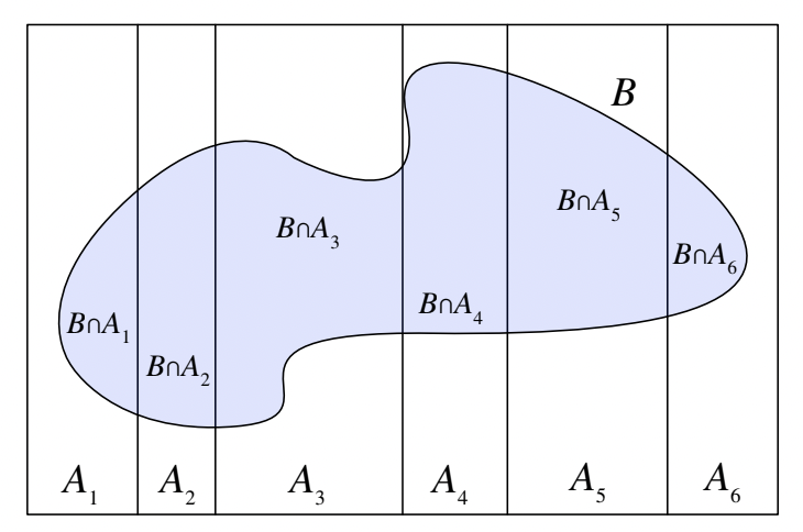
Fig. 2.3 Visualization of the law of total probability. This is Figure 2.3 from [BH19].

Law of total probability (LOTP).

Suppose \(A_1, \dots, A_n\) partition sample space \(S\), which means that they’re disjoint their union is \(S\), as in Figure 2.3. The law of total probability tells us that

\[\begin{equation*} \mathbb{P}[B] = \sum_{i = 1}^n \mathbb{P}[B \cap A_i] = \sum_{i = 1}^n \mathbb{P}[B \mid A_i] \mathbb{P}[A_i]. \end{equation*}\]

Example: The importance of scoring first.

This example is from [Sev20].

Using data from the English Premier League, we can calculate the probability that the home team wins by considering different scenarios regarding which team scores first. In particular, we can use LOTP to derive the following formula:

\[\begin{align*} &\mathbb{P}[\text{home team wins}]\\ =\, &\mathbb{P}[\text{home team wins} \mid \text{home team scores first}] \cdot \mathbb{P}[\text{home team scores first}]\\ +\, &\mathbb{P}[\text{home team wins} \mid \text{visitor scores first}] \cdot \mathbb{P}[\text{visitor scores first}]\\ +\, &\mathbb{P}[\text{home team wins} \mid \text{neither team scores first}] \cdot \mathbb{P}[\text{neither team scores first}]. \end{align*}\]

From the EPL data, we have the following values:

• \(\mathbb{P}[\text{home team wins} \mid \text{home team scores first}] = 0.718\)

• \(\mathbb{P}[\text{home team scores first}] = 0.534\)

• \(\mathbb{P}[\text{home team wins} \mid \text{visitor scores first}] = 0.178\)

• \(\mathbb{P}[\text{visitor scores first}] = 0.39\)

• \(\mathbb{P}[\text{home team wins} \mid \text{neither team scores first}] = 0\)

• \(\mathbb{P}[\text{neither team scores first}] = 0.076\)

Using these values, the total probability of the home team winning is: \(0.718 \cdot 0.534 + 0.178 \cdot 0.39 + 0 \cdot 0.076 = 0.453\).

We’ll now work through an example that combines Bayes’ rule and LOTP. Suppose we have a population of 10 sick and 90 healthy people, as in the following figure.

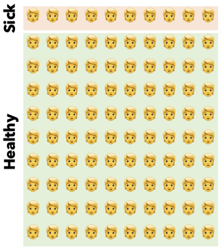
Fig. 2.4 10 sick and 90 healthy people.

If we chose a random person from this pool,

\[\begin{equation*} \mathbb{P}[\text{random person is sick}] = \frac{\text{(# sick)}}{\text{# total people}} = \frac{10}{100}. \end{equation*}\]

Now, suppose that we test this population. Of the 10 sick people, suppose that 9 test positive, and of the 90 healthy people, another 9 test positive, as in the following figure.

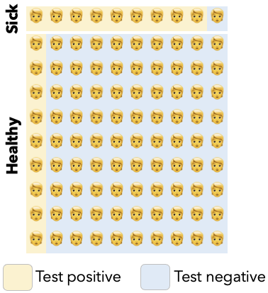
Fig. 2.5 Results of a test.

If we chose a random sick person from this pool, the probability they test positive is:

\[\begin{align*} \mathbb{P}[\text{random person tests positive} \mid \text{they’re sick}] &= \frac{\text{(# people who are sick and test positive)}}{\text{(# sick people)}}\\ &= \frac{9}{10}. \end{align*}\]

Meanwhile, suppose we chose a random person from this pool who tested positive, as highlighted in the following figure.

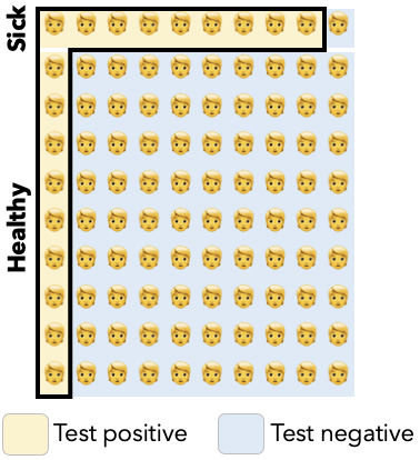
Fig. 2.6 Highlighting the people who tested positive, both sick and healthy.

The probability they’re actually sick is equal to

\[\begin{align*} \mathbb{P}[\text{random person is sick} \mid \text{they test positive}] &= \frac{\text{(# people who are sick and test positive)}}{\text{(# people who test positive)}}\\ &= \frac{9}{18} = \frac{1}{2}. \end{align*}\]

In other words, even if you tested positive, you only have a 50-50 chance of being sick! This surprising fact is called the “false positive paradox.”

Another way to express this probability is via Bayes’ rule:

\[\begin{align*} \mathbb{P}[\text{random person is sick} \mid \text{they test positive}] &= \frac{\mathbb{P}[\text{positive} \mid \text{sick}]\mathbb{P}[\text{sick}]}{\mathbb{P}[\text{positive}]}\\ &= \frac{\frac{9}{10} \cdot \frac{1}{10}}{\frac{18}{100}} = \frac{1}{2}. \end{align*}\]

To get an intuition for the false positive paradox, we will expand out the denominator of this equation using the LOTP:

\[\begin{align*} &\mathbb{P}[\text{random person is sick} \mid \text{they test positive}]\\ =\, &\frac{\mathbb{P}[\text{positive} \mid \text{sick}]\mathbb{P}[\text{sick}]}{\mathbb{P}[\text{positive} \mid \text{sick}]\mathbb{P}[\text{sick}] + \mathbb{P}[\text{positive} \mid \text{healthy}]\mathbb{P}[\text{healthy}]}. \end{align*}\]

We can see that as \(\mathbb{P}[\text{healthy}]\) gets larger and larger, the \(\mathbb{P}[\text{random person is sick} \mid \text{they test positive}]\) will get smaller and smaller. Intuitively, once a significant fraction of the population is healthy, a relatively large number will test positive compared to the true positives, and \(\mathbb{P}[\text{random person is sick} \mid \text{they test positive}]\) will be driven to a small number.

We’ll finish this section with a few more examples.

Example

This example is from [Ros18].

Imagine you’re going away for the weekend and ask your roommate to water your plant. If your roommate forgets to water the plant, there’s a 90% chance it will be dead by the time you return. If your roommate remembers to water the plant, there’s only a 10% chance it will die. You’re fairly confident that your roommate will remember to water it, estimating the likelihood at 85%.

Question 1: What is the probability that your plant will still be alive when you return?

Step 1: Define the events. Let’s define the events:

• \( R \): Your roommate waters the plant.

• \( D \): The plant is dead.

Step 2: Define the goal. To answer the question, we want to calculate \( \mathbb{P}[D^c] \), the probability that the plant is not dead, using the Law of Total Probability:

\[\begin{equation*} \mathbb{P}[D^c] = \mathbb{P}[D^c \mid R] \cdot \mathbb{P}[R] + \mathbb{P}[D^c \mid R^c] \cdot \mathbb{P}[R^c] \end{equation*}\]

Step 3: Compute the individual probabilities. We are given the following information:

• \( \mathbb{P}[D \mid R^c] = 0.9 \), so \( \mathbb{P}[D^c \mid R^c] = 0.1 \).

• \( \mathbb{P}[D \mid R] = 0.1 \), so \( \mathbb{P}[D^c \mid R] = 0.9 \).

• \( \mathbb{P}[R] = 0.85 \), meaning your confidence in your roommate remembering is 85%.

Step 4: Plug in to get the final answer. Now we can calculate the probability that the plant is alive:

\[\begin{equation*} \mathbb{P}[D^c] = 0.9 \cdot 0.85 + 0.1 \cdot 0.15 = 0.78. \end{equation*}\]

---

Question 2: You return home to find your plant is dead. What is the probability that your roommate forgot to water it?

In other words, we want to calculate \( \mathbb{P}[R^c \mid D] \), the probability that your roommate forgot, given that the plant is dead.

Using Bayes’ Rule:

\[\begin{equation*} \mathbb{P}[R^c \mid D] = \frac{\mathbb{P}[D \mid R^c] \cdot \mathbb{P}[R^c]}{\mathbb{P}[D]} = \frac{\mathbb{P}[D \mid R^c] \cdot \mathbb{P}[R^c]}{1 - \mathbb{P}[D^c]} \end{equation*}\]

From the previous information, we know:

• \( \mathbb{P}[D \mid R^c] = 0.9 \)

• \( \mathbb{P}[R^c] = 0.15 \) (since \( \mathbb{P}[R] = 0.85 \))

• \( \mathbb{P}[D^c] = 0.78 \), so \( \mathbb{P}[D] = 1 - 0.78 = 0.22 \)

Now, plugging in the values:

\[\begin{equation*} \mathbb{P}[R^c \mid D] = \frac{0.9 \cdot 0.15}{0.22} \approx 0.61. \end{equation*}\]

Example

This example is from [HB23].

Imagine a bomb detector system where the alarm lights up with high accuracy if a bomb is present. Specifically, if a bomb is there, the alarm goes off with a probability of 0.99. However, the system isn’t perfect, and if no bomb is present, the alarm still (incorrectly) lights up with a probability of 0.05. Additionally, suppose that the likelihood of a bomb being present in any given situation is 0.1.

Question: Given that the alarm has gone off, what is the probability that there is actually a bomb?

Step 1: Define the events.

• \( A \): The alarm goes off.

• \( B \): A bomb is present.

Step 2: Define the goal. To answer the question, we need to calculate \( \mathbb{P}[B \mid A] \), the probability that a bomb is present given that the alarm has gone off. We can use Bayes’ Rule for this calculation:

\[\begin{equation*} \mathbb{P}[B \mid A] = \frac{\mathbb{P}[A \mid B] \cdot \mathbb{P}[B]}{\mathbb{P}[A]} \end{equation*}\]

Step 3: Compute the individual probabilities. From the given information, we know:

• \( \mathbb{P}[A \mid B] = 0.99 \) (the probability that the alarm goes off if a bomb is present).

• \( \mathbb{P}[A \mid B^c] = 0.05 \) (the probability that the alarm goes off when there is no bomb).

• \( \mathbb{P}[B] = 0.1 \) (the probability that a bomb is present).

• \( \mathbb{P}[B^c] = 0.9 \) (the probability that there is no bomb).

Step 4: Plug in to get the final answer. Now, we can calculate the desired probability:

\[\begin{equation*} \mathbb{P}[B \mid A] = \frac{\mathbb{P}[A \mid B] \cdot \mathbb{P}[B]}{\mathbb{P}[A \mid B] \cdot \mathbb{P}[B] + \mathbb{P}[A \mid B^c] \cdot \mathbb{P}[B^c]}. \end{equation*}\]

Substituting the known values:

\[\begin{equation*} \mathbb{P}[B \mid A] = \frac{0.99 \cdot 0.1}{0.99 \cdot 0.1 + 0.05 \cdot 0.9} = \frac{0.099}{0.099 + 0.045} = \frac{0.099}{0.144} \approx 0.6875. \end{equation*}\]

2.3. Independence

In probability theory, we’ve observed several examples where conditioning on one event alters the probability of other events. In this section, we will focus on independence, where the occurrence of one event provides no information about the occurrence of another.

Independence.

Two events \( A \) and \( B \) are independent if the probability of both events occurring together equals the product of their individual probabilities, i.e., \(\mathbb{P}[A \cap B] = \mathbb{P}[A]\mathbb{P}[B].\)

This can be rewritten as:

\[\begin{equation*} \mathbb{P}[A \mid B] = \frac{\mathbb{P}[A \cap B]}{\mathbb{P}[B]} = \mathbb{P}[A]. \end{equation*}\]

In other words, knowing whether \( B \) has occurred does not provide any information about whether \( A \) has occurred.

Independence of three events.

For three events \( A \), \( B \), and \( C \), independence means that:

1. \( \mathbb{P}[A \cap B] = \mathbb{P}[A]\mathbb{P}[B] \), \( \mathbb{P}[A \cap C] = \mathbb{P}[A]\mathbb{P}[C] \), and \( \mathbb{P}[B \cap C] = \mathbb{P}[B]\mathbb{P}[C]\), and

2. \(\mathbb{P}[A \cap B \cap C] = \mathbb{P}[A]\mathbb{P}[B]\mathbb{P}[C].\)

It’s important to note that pairwise independence (condition 1) does not necessarily imply joint independence (condition 2).

Conditional independence.

Two events \( A \) and \( B \) are conditionally independent given a third event \( E \) if \(\mathbb{P}[A \cap B \mid E] = \mathbb{P}[A \mid E]\mathbb{P}[B \mid E].\) This means that, given \( E \), the occurrence of \( A \) provides no further information about the occurrence of \( B \), and vice versa.

As the following examples illustrate, independence does not necessarily imply conditional independence, and vice versa.

Example: Conditional independence doesn’t imply independence.

Consider a scenario where a box contains two coins: Coin 1 is a regular coin with one head and one tail, while Coin 2 is a special coin with two heads. One of these coins is randomly chosen, and it is flipped twice.

Let the event \( A = \{HH, HT\}\) represent the outcome where the first toss results in heads (H), and \( B = \{HH, TH\}\) represent the event where the second toss results in heads. Additionally, let \( E \) denote the event that Coin 1 was chosen.

Conditional independence. Given that Coin 1 (a regular coin) is chosen, the events \( A \) and \( B \) are conditionally independent. This is because, for Coin 1, the probability of getting heads on either toss is \( \frac{1}{2} \). Therefore, the conditional probabilities are \(\mathbb{P}[A \mid E] = \mathbb{P}[\{HH, HT\} \mid \text{Coin 1 chosen}] = \frac{1}{2}\). Similarly, \(\mathbb{P}[B \mid E] = \frac{1}{2}.\) Additionally, the probability of both tosses resulting in heads, given that Coin 1 was chosen, is \(\mathbb{P}[A \cap B \mid E] = \mathbb{P}[\{HH\} \mid \text{Coin 1 chosen}] = \frac{1}{4}\). Thus, \( A \) and \( B \) are independent events conditioned on choosing Coin 1 because \(\mathbb{P}[A \cap B \mid E] = \mathbb{P}[A \mid E] \cdot \mathbb{P}[B \mid E]\).

Unconditional dependence. However, \( A \) and \( B \) are not independent when we don’t condition on \( E \). By the law of total probability, \(\mathbb{P}[B] = \mathbb{P}[B \mid E]\cdot \mathbb{P}[E] + \mathbb{P}[B \mid E^c]\cdot \mathbb{P}[E^c]\). We’ve already computed \(\mathbb{P}[B \mid E] = \frac{1}{2}\), and we know that \(\mathbb{P}[E] = \frac{1}{2}\), so \(\mathbb{P}[E^c] = \mathbb{P}[\text{Coin 2 chosen}] = \frac{1}{2}\) as well. If Coin 2 is chosen, HH is the only possible outcome. Therefore, \(\mathbb{P}[B \mid E^c] = \mathbb{P}[\text{HH or TH} \mid \text{Coin 2 chosen}] = 1.\) Putting this all together, we have that

\[\begin{equation*} \mathbb{P}[B] = \frac{1}{2} \cdot \frac{1}{2} + 1 \cdot \frac{1}{2} = \frac{3}{4}. \end{equation*}\]

By the same logic, \(\mathbb{P}[A] = \frac{3}{4}\). Meanwhile, the probability both tosses land heads (\(A \cap B = \{HH\}\)) is:

\[\begin{equation*} \mathbb{P}[A \cap B] = \mathbb{P}[A \cap B \mid E]\cdot \mathbb{P}[E] + \mathbb{P}[A \cap B \mid E^c]\cdot \mathbb{P}[E^c] = \frac{1}{4} \cdot \frac{1}{2} + 1 \cdot \frac{1}{2} = \frac{5}{8}. \end{equation*}\]

Since \( \mathbb{P}[A] \mathbb{P}[B] \neq \mathbb{P}[A \cap B] \), we conclude that \( A \) and \( B \) are not independent events when we don’t know which coin was chosen. Intuitively, if the first flip lands heads (i.e., \(A\) happens), we can assume there’s a good chance we chose Coin 2, and therefore, there’s a higher likelihood that the second flip will land heads as well. Said another way, given that \(A\) happens, we can be slightly more confident that \(B\) will also happen.

Example: Independence doesn’t imply conditional independence.

Suppose my friends Alice and Bob each decide, independently of one another, whether or not to call me every day. Let’s define a few events: \( A \) represents the event that Alice calls this coming Friday, and \( B \) represents the event that Bob calls this coming Friday. Additionally, let \( E \) denote the event that I receive exactly one call this coming Friday.

Given that I receive exactly one call (\( E \)), either Alice or Bob may be the one who calls, so the probabilities \( \mathbb{P}[A \mid E]\) and \( \mathbb{P}[B \mid E]\) are non-zero (i.e., \( \mathbb{P}[A \mid E] > 0 \) and \( \mathbb{P}[B \mid E] > 0 \)).

However, the probability of both Alice and Bob calling, given that I receive exactly one call, is zero: \(\mathbb{P}[A \cap B \mid E] = 0.\) Therefore, \(0 = \mathbb{P}[A \cap B \mid E] \not= \mathbb{P}[A \mid E] \cdot \mathbb{P}[B \mid E] > 0\), so \(A\) and \(B\) are not conditionally independent, given \(E\).

2.4. The Monty Hall problem

We’ll now see how working with conditional probability can help us solve a famous problem from the game show Let’s Make a Deal, hosted by Monty Hall. On this show, a contestant plays a game involving three doors: behind one of the doors is a car, while the other two doors conceal goats. Each door conceals the car with equal probability.

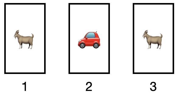
Fig. 2.7 Three doors. One conceals a car and the others conceal goats.

Monty, the game show host, knows which door hides the car and which doors hide the goats. Here’s how the game works:

1. The contestant begins by choosing one of the three doors. Next, Monty will open one of the other two doors. Importantly, Monty will always open a door that hides a goat. If both of the remaining doors have goats behind them, Monty will choose which door to open with equal probabilities.

2. After Monty opens the door, revealing a goat, the contestant is given a choice: either stick with their original door or switch to the remaining unopened door.

3. Finally, Monty will open the contestant’s chosen door, and the contestant will win whatever is behind it, either the car or a goat.

The contestant has two possible strategies to choose from in the game:

1. Switch: The contestant initially selects door 1 (without loss of generality). After Monty opens a door revealing a goat, the contestant switches to the other remaining door.

2. Stay: The contestant selects door 1, and after Monty opens a door revealing a goat, they stick with their original choice and keep door 1.

Q1: What is the probability the contestant wins under the “stay” strategy?

In this case, the contestant will only win if the car is behind door 1, so the probability they win is \(\frac{1}{3}\) (since the car is behind each door with equal probability).

Q2: What is the probability the contestant wins under the “switch” strategy?

Step 1: Define the events. We start by defining the relevant events in the game. Let:

• \( A \) be the event you win the car if you switch doors.

• \( C_j \) be the event that the car is behind door \( j \), where \( j = 1, 2, 3 \).

Step 2: Define the goal. We aim to calculate the probability of winning the car if you switch, denoted as \( \mathbb{P}[A] \). We use the Law of Total Probability (LOTP) to break this down into conditional probabilities based on where the car is located: \(\mathbb{P}[A] = \mathbb{P}[A \mid C_1]\mathbb{P}[C_1] + \mathbb{P}[A \mid C_2]\mathbb{P}[C_2] + \mathbb{P}[A \mid C_3]\mathbb{P}[C_3].\)

Step 3: Calculate the individual probabilities. Now, we compute the individual probabilities:

• The probability of the car being behind any of the three doors is equally likely, so \(\mathbb{P}[C_1] = \mathbb{P}[C_2] = \mathbb{P}[C_3] = \frac{1}{3}.\)

• If the car is behind door 1 (\( C_1 \)), switching will result in a loss, so \(\mathbb{P}[A \mid C_1] = 0.\)

• If the car is behind door 2 (\( C_2 \)), Monty will open door 3. Therefore, you will switch to door 2 and win the car, so \(\mathbb{P}[A \mid C_2] = 1.\)

• Similarly, if the car is behind door 3 (\( C_3 \)), Monty will open door 2. Therefore, you will switch to door 3 and win the car, so \(\mathbb{P}[A \mid C_3] = 1.\)

Step 4: Compute the final answer. Using these values, we can now compute the overall probability of winning by switching: \(\mathbb{P}[A] = 0 \cdot \frac{1}{3} + 1 \cdot \frac{1}{3} + 1 \cdot \frac{1}{3} = \frac{2}{3}.\) Therefore, the probability of winning the car if you switch doors is \( \frac{2}{3} \), which makes switching the optimal strategy in the Monty Hall problem.

Tree diagrams can help us work through slightly more complex probabilities. For example, let \(M_j\) be the event that Monty opens door \(j\), for \(j = 1, 2, 3\).

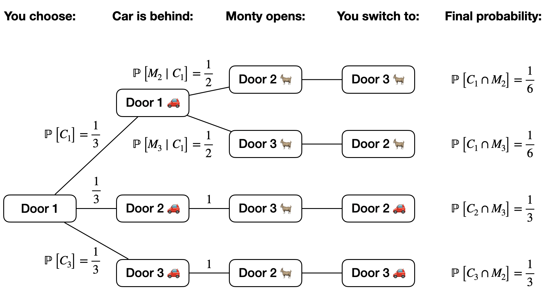
Fig. 2.8 Tree diagram for the Monty hall problem.

Q: What is the probability you win if you switch, given that Monty opens door 2? In other words, let \(A\) be the event you win if you switch. What is \(\mathbb{P}[A \mid M_2]\)?

We know that

\[\begin{equation*} \mathbb{P}[A \mid M_2] = \frac{\mathbb{P}[A \cap M_2]}{\mathbb{P}[M_2]}. \end{equation*}\]

The only way that you can win if you switch in the scenario that Monty opens door 2 is if the car is behind door 3. Therefore, the event \(A \cap M_2\) is equivalent to the event \(C_3 \cap M_2\). Figure 2.8 illustrates that \(\mathbb{P}[C_3 \cap M_2] = \frac{1}{3}\).

Meanwhile, by the law of total probability, \(\mathbb{P}[M_2] = \mathbb{P}[M_2 \cap C_1] + \mathbb{P}[M_2 \cap C_2] + \mathbb{P}[M_2 \cap C_3]\). Note that \(\mathbb{P}[M_2 \cap C_2] = 0\), since Monty will never open a door that has a car behind it. From Figure 2.8, we see that \(\mathbb{P}[M_2 \cap C_1] = \frac{1}{6}\) and \(\mathbb{P}[M_2 \cap C_3] = \frac{1}{3}\). Therefore,

\[\begin{equation*} \mathbb{P}[A \mid M_2] = \frac{\mathbb{P}[C_3 \cap M_2]}{\mathbb{P}[M_2]} = \frac{1/3}{1/6 + 1/3} = \frac{2}{3}. \end{equation*}\]

So even if you condition on Monty opening door 2, you still have a \(\frac{2}{3}\) probability of winning under the switching strategy.

2.5. Paradoxes and fallacies

We will end this chapter with some famous paradoxes from probability.

2.5.1. Prosecutor’s fallacy

In 1998, Sally Clark was tried for the murder of her two sons, both of whom tragically died as infants. During the trial, the prosecutor argued that the probability of a newborn dying from sudden infant death syndrome (SIDS) was 1 in 8500. Based on this, they claimed that the probability of Clark being innocent was \( \frac{1}{8500^2} \).

However, this reasoning contained two significant flaws. First, it assumed the deaths were independent events, which may not be the case: genetic factors could link the deaths, making them not independent. Second, and more crucially, the prosecutor misapplied probability. They claimed that the likelihood of the evidence (the deaths of the children) given Clark’s innocence was \( \frac{1}{8500^2} \). However, what we actually what to determine is the probability of Clark being innocent given the evidence — a fundamentally different quantity.

As we know from Bayes’ rule,

\[\begin{equation*} \mathbb{P}[\text{innocent} \mid \text{evidence}] = \frac{\mathbb{P}[\text{evidence} \mid \text{innocent}] \cdot \mathbb{P}[\text{innocent}]}{\mathbb{P}[\text{evidence}]}. \end{equation*}\]

Expanding it further with the LOTP:

\[\begin{equation*} \mathbb{P}[\text{innocent} \mid \text{evidence}] = \frac{\mathbb{P}[\text{evidence} \mid \text{innocent}] \cdot \mathbb{P}[\text{innocent}]}{\mathbb{P}[\text{evidence} \mid \text{innocent}] \cdot \mathbb{P}[\text{innocent}] + \mathbb{P}[\text{evidence} \mid \text{guilty}] \cdot \mathbb{P}[\text{guilty}]}. \end{equation*}\]

This equation shows that if the probability of guilt is sufficiently small, then the probability of innocence, given the evidence, would be close to 1. Therefore, the prosecutor’s simplistic approach vastly overstated the likelihood of guilt by failing to apply the correct probabilistic reasoning. This mistake is commonly referred to as the “prosecutor’s fallacy.”

2.5.2. Simpson’s paradox

Simpson’s paradox is a phenomenon in probability where a trend that appears in different groups of data reverses when the groups are combined. We’ll see two examples of this paradox.

Table 2.1 Survival data of 100 people from Country A

	Young	Old
Survived	10	70
Didn’t survive	0	20

Table 2.2 Survival data of 100 people from Country B

	Young	Old
Survived	81	2
Didn’t survive	9	8

Example: Disease survival rates.

Simpson’s paradox can be illustrated through an example involving disease survival rates in two countries, Country A and Country B. The survival data for both countries is shown in Table 2.1 and Table 2.2.

At first glance, when we calculate the overall survival rates, Country B appears to have a slightly higher survival rate (83%) than Country A (80%). However, this conclusion is deceptive. When the data is conditioned on age, Country A has a better survival rate for both young and old patients.

To write this in terms of probability, let \(L\) be the event that a randomly chosen patient survives the disease. Let \(A\) be the event that the patient lives in country A and \(B\) be the event that they live in country B. Moreover, let \(Y\) be the event that the patient is young. We denote the probability the patient survives given that they live in country A and are young as \(\mathbb{P}[L \mid A , Y]\), a common shorthand for \(\mathbb{P}[L \mid A \cap Y]\). We have that \(\mathbb{P}[L \mid A, Y]= 1.0 > \mathbb{P}[L \mid B, Y] = \frac{81}{90}\) and \(\mathbb{P}[L \mid A, Y^c] = \frac{70}{90} > \mathbb{P}[L \mid B, Y^c] = \frac{2}{10}\). However, \(\mathbb{P}[L \mid A] = \frac{80}{100} < \mathbb{P}[L \mid B] = \frac{83}{100}.\)

This paradox occurs because the age distributions of the two countries are different. Country A has a larger proportion of elderly patients, and many survive (for example, due to excellent elder care). In contrast, Country B has fewer elderly patients, but perhaps the care for older individuals is poor, resulting in a lower survival rate. However, the younger population in Country B is relatively large and has a high survival rate, skewing the overall survival statistics.

Thus, while Country B appears to have a better overall survival rate, Country A performs better when we examine the data separately by age group. This reversal of conclusions, depending on how the data is grouped, is a classic example of Simpson’s paradox.

Example: Batting average against.

In 2009, pitchers Beckett and Santana had very similar batting averages against (BAA), the percentage of at-bats that result in a hit by the opposing team’s batters. Lower is better since the BAA measures how effectively a pitcher prevents hits. Beckett’s BAA was 0.2441, and Santana’s was 0.2438. To write these numbers in terms of events, let \( H_B \) be the event that Beckett allows a hit, with \( \mathbb{P}[H_B] = 0.2441 \). Similarly, let \(H_S\) be the event Santana allows a hit, with \( \mathbb{P}[H_S] = 0.2438 \).

However, when we break down the data by handedness of the batters, Beckett’s performance appears better. Let \( R_B \) be the event that a batter facing Beckett was right-handed, and let \(R_S\) be the same for Santana. For right-handed batters, Beckett’s conditional BAA was \( \mathbb{P}[H_B \mid R_B] = 0.226 \), while Santana’s was \( \mathbb{P}[H_S \mid R_S] = 0.235 \). Similarly, against left-handed batters, Beckett’s BAA was \( \mathbb{P}[H_B \mid R_B^c] = 0.258 \), compared to Santana’s \( \mathbb{P}[H_S \mid R_S^c] = 0.267 \). Despite these superior conditional BAAs for Beckett, his overall BAA was slightly worse than Santana’s.

This difference arises from the distribution of right- and left-handed batters each pitcher faced. Beckett faced a lower proportion of right-handed batters compared to Santana. Using the LOTP, the overall BAA can be calculated by considering both conditional probabilities and the proportions of right- and left-handed batters faced:

\[\begin{align*} \mathbb{P}[H_B] &= \mathbb{P}[H_B \mid R_B]\mathbb{P}[R_B] + \mathbb{P}[H_B \mid R_B^c]\mathbb{P}[R_B^c]\\ &= 0.226 \times 0.432 + 0.258 \times 0.568 = 0.2441 \end{align*}\]

and

\[\begin{align*} \mathbb{P}[H_S] &= \mathbb{P}[H_S \mid R_S]\mathbb{P}[R_S] + \mathbb{P}[H_S \mid R_S^c]\mathbb{P}[R_S^c]\\ &= 0.235 \times 0.719 + 0.267 \times 0.281 = 0.2438. \end{align*}\]

Santana faced a significantly higher proportion of right-handed batters (71.9%) compared to Beckett (43.2%), which contributed to lowering his overall BAA, despite his conditional BAAs being worse than Beckett’s in both right- and left-handed matchups.