1. Probability and counting

1.1. Sets

In probability, the primary goal is to determine how likely a specific set of outcomes is, given a particular experiment. In this section, we’ll focus on understanding the concept of sets, which form the foundation of probability theory.

A set is a collection of objects or elements. For example, the set \(\{1, 3, 5, 7\}\) contains four numbers, while the outcomes from flipping a coin twice form the set \(\{HH, HT, TH, TT\}\) (where \(H\) stands for Heads and \(T\) stands for Tails). There’s also the empty set, denoted \(∅\), which contains no elements.

Subsets. If every element in the set \(A\) is also in the set \(B\), then \(A\) is called a subset of \(B\), represented as \(A \subseteq B\). For example, \(\{HH, HT\} \subseteq \{HH, HT, TH, TT\}\).

Elements of sets. When we use the notation \(a \in A\), it means that \(a\) is an element of set \(A\). Meanwhile, the notation \(a \notin A\) means that \(a\) is not an element of \(A\). For example, \(1 \in \{1, 3, 5, 7\}\), but \(2 \notin \{1, 3, 5, 7\}\).

Unions and intersections. Key operations involving sets include the union and intersection. The union of two sets, denoted \(A \cup B\), is the set of elements that are in either \(A\) or \(B\), or both. See Figure 1.1 for an illustration.

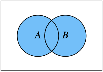
Fig. 1.1 Union \(A\cup B\)

The intersection, \(A \cap B\), contains the elements that are in both sets, as in Figure 1.2.

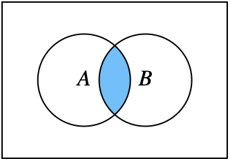
Fig. 1.2 Intersection \(A \cap B\)

If two sets share no elements, they are called disjoint, meaning \(A \cap B = \emptyset\), as in Figure 1.3.

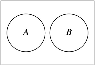
Fig. 1.3 Disjoint sets

Complements. Often, we work with sets that are part of a larger set, called a sample space. The complement of a set \(A\), denoted \(A^c\), consists of elements in the sample space that are not in \(A\), as illustrated in Figure 1.4.

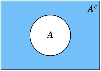
Fig. 1.4 Complement \(A^c\)

Cardinality. The final definition we’ll cover in this section is the cardinality of a set, which is the number of elements in the set, denoted \(|A|\). For example, if \(A = \{1, 3, 5, 7\}\), then \(|A| = 4\).

1.2. Sample spaces and events

The sample space of an experiment, typically denoted as \(S\), is the set of all possible outcomes of that experiment. For instance, if our experiment involves flipping two coins, the sample space is \(\{HH, HT, TH, TT\}\). An event is a subset of the sample space. For example, the event that exactly one coin lands Heads is represented by the subset \(\{HT, TH\}\).

Example: Deck of cards

This is Example 1.2.3 by [BH19].

Suppose we have a standard deck of 52 cards, and our experiment is drawing a single card. In this case, the sample space \(S\) is the set of all 52 cards. We can define many events based on this experiment. For example:

• Let \(A\) be the event that the card drawn is an ace. In other words,
  \(A = \{\text{Ace of Diamonds, Ace of Clubs, Ace of Hearts, Ace of Spades}\}\), and \(|A| = 4\).

• Let \(B\) be the event that the card drawn has a black suit (i.e., clubs or spades).

• Let \(C\) be the event that the card drawn is a diamond.

• Let \(D\) be the event that the card drawn is a heart.

We can also define intersections and unions of events. For example:

• \(A \cap D\) is the event that the card is the Ace of Hearts.

• \(A \cap B\) is the event that the card is either the Ace of Spades or the Ace of Clubs.

• \(A \cup C \cup D\) is the event that the card is either red (i.e., it is a diamond or heart) or an ace.

• Finally, \((A \cup B)^c = A^c \cap B^c\) is the event that the card is a red non-ace.

Example: Soccer

Suppose our experiment is a soccer match where Arsenal plays Liverpool. In this case, the sample space \(S = \{\text{Arsenal wins, Liverpool wins, draw}\}\) is the set of possible outcomes. We could define the event \(A\) to capture the scenario where Arsenal doesn’t win, i.e., \(A = \{\text{Liverpool wins, draw}\}\).

Example: Stocks

We can also view a stock’s performance over time as an experiment. For example, suppose we track its price over the course of a month. A simple example of a sample space for this experiment would be \(S = \{\text{price goes up, price goes down, price stays the same}\}\). We could define the event \(A\) to capture the scenario where the stock price doesn’t go up, i.e., \(A = \{\text{price goes down, price stays the same}\}\).

1.3. A naive definition of probability

As described at the beginning, the primary goal in probability is to determine how likely a specific set of outcomes is, given a particular experiment. Given an event \(A\) (such as Arsenal not winning a match or a stock price not rising), our goal will be to determine how likely that event is to occur. We will refer to this likelihood as the probability of the event \(A\).

In this section, we will begin with a very basic, naive method for calculating the probability of the event \(A\), which we will denote as \(\mathbb{P}_{\text{naive}}[A]\). This method is only to build intuition. Later in this chapter, with this intuition, we will be ready to move on to the actual, non-naive definition of probability.

The first method you might try to calculate the likelihood of an event \(A\) is to count the number of outcomes where that event happens—which we will call the number of “favorable” outcomes—and divide it by the total number of possible outcomes. Since \(A\) is a set of outcomes, we know that the number of favorable outcomes is \(|A|\) and the number of possible outcomes is the size of the sample space \(|S|\). In other words,

\[\begin{equation*} \mathbb{P}_{\text{naive}}[A] = \frac{\# \text{favorable outcomes}}{\# \text{possible outcomes}} = \frac{|A|}{|S|}. \end{equation*}\]

For example, suppose we flip two coins, and \(A = \{HT, TH\}\) is the event that exactly one Head appears. Then

\[\begin{equation*} \mathbb{P}_{\text{naive}}[A] = \frac{|A|}{|S|} = \frac{2}{4}. \end{equation*}\]

Intuitively, this makes sense!

Similarly, suppose we pick a card from a standard deck. Let \(A\) be the event that we draw the Ace of Spades or the Ace of Clubs. Then

\[\begin{equation*} \mathbb{P}_{\text{naive}}[A] = \frac{|A|}{|S|} = \frac{2}{52}. \end{equation*}\]

Remember that the complement of \(A\), denoted \(A^c\), consists of the elements in the sample space that are not in \(A\). Therefore, the probability that event \(A\) does not happen is \(\mathbb{P}_{\text{naive}}[A^c]\), which we can calculate as:

\[\begin{equation*} \mathbb{P}_{\text{naive}}[A^c] = \frac{|A^c|}{|S|} = \frac{|S| - |A|}{|S|} = 1 - \mathbb{P}_{\text{naive}}[A]. \end{equation*}\]

This naive approach to probability assumes that all outcomes are equally likely and that the number of possible outcomes is finite. However, in many cases, such as predicting the outcome of a soccer match, not all outcomes are equally likely (e.g., Arsenal winning versus Liverpool winning). Therefore, we will require a more sophisticated approach to calculating probabilities, which we will introduce later in this chapter.

1.4. Counting

To use the naive definition of probability introduced above, we need to be able to count the number of favorable outcomes of an experiment \(|A|\), as well as the total number of possible outcomes \(|S|\). This is straightforward in the examples we’ve seen so far, but it becomes challenging for complex experiments. In this section, we will develop tools for calculating the sizes of sets.

1.4.1. Multiplication rule

We will begin with the simple multiplication rule. Suppose we run an experiment with two parts, \(C\) and \(D\). Suppose \(C\) has \(c\) possible outcomes, and for each possible outcome of \(C\), there are \(d\) possible outcomes of \(D\). The multiplication rule tells us that this experiment has a total of \(c \cdot d\) outcomes.

Example: Running a race

Suppose Alice, Bob, Claire, and David are running a race. Our “experiment” is determining who will win first and second place. Thus, the outcome of this experiment has two parts: the first-place winner and the second-place winner. There are four possibilities for the first-place winner, and once that outcome is determined, there are three possibilities for the second-place winner (for example, if Alice wins first place, then Bob, Claire, or David could win second place). Therefore, this experiment’s total number of outcomes (again, determining who wins first and second place) is \(4 \cdot 3 = 12\).

These outcomes can be visualized with the tree diagram in Figure 1.5, where the first level indicates possible first-place winners, and the second level indicates possible second-place winners. The tree has a total of 12 leaves, corresponding to the 12 possible outcomes of the experiment.

Fig. 1.5 Possible first- and second-place finishers.

We can extend the logic in this example to the following general rule.

General rule

If we have \(n\) objects, there are \(n! = n \cdot (n-1) \cdot (n-2) \cdots 2 \cdot 1\) ways to order those objects.

Example: Assigning majors to students.

Suppose we have five majors—-BioE, CS, CE, EE, and MS&E—-and three students—-Alice, Bob, and Claire. How many ways are there to assign majors to these students? The answer is \(5 \cdot 5 \cdot 5\) because there are five ways to assign a major to Alice, five ways to assign a major to Bob, and so on. Unlike the previous example, the major we assign to Alice doesn’t limit the majors we can assign to Bob or Claire (so the answer is not \(5 \cdot 4 \cdot 3\)).

However, suppose we wanted to assign a unique major to each student. There would be \(5 \cdot 4 \cdot 3\) possible ways to do so, since there would be five ways to assign a major to Alice, and once her major has been determined, four ways to assign a different major to Bob, and then finally three ways to assign a major to Claire that is different from Alice and Bob’s.

Example: The birthday paradox.

This is a famous example (Example 1.4.10 from [BH19]) of the multiplication rule. Suppose we have \(k\) people in a room, each of whom is equally likely to be born on any of the 365 days of the year. Our goal is to determine the probability that at least two people in the room share the same birthday. We will work with our naive definition of probability to answer this question, but fortunately in this case, the naive probability will be the true probability!

In this class, I aim to give you a step-by-step guide to solving these types of problems, which will serve you well in the homeworks and exams.

Step 1: Define the events. To solve this problem, we begin by defining the relevant events:

• Let \(A\) represent the event that at least one pair has the same birthday.

• Let \(A^c\) represent the complement, which is the event that all \(k\) people have different birthdays.

Step 2: Define the goal. Our goal is to calculate the probability \(\mathbb{P}_{\text{naive}}[A]\), which, as we saw earlier in this chapter, is equal to \(1 - \mathbb{P}_{\text{naive}}[A^c]\). By definition,

\[\begin{align*} \mathbb{P}_{\text{naive}}[A^c] &= \frac{\text{# of favorable outcomes}}{\text{# of possible outcomes}}\\ &= \frac{\text{# of ways to assign birthdays so all $k$ people have different birthdays}}{\text{Total # of ways to assign birthdays to $k$ people}}. \end{align*}\]

Step 3: Calculate the relevant quantities. Now, we calculate the number of possible outcomes and favorable outcomes:

• Number of possible outcomes: Since each person can have any of the 365 days as their birthday, the total number of ways to assign birthdays to \(k\) people is

\[\begin{equation*}\underbrace{365 \cdot 365 \cdots 365}_{k \text{ times}} = 365^k.\end{equation*}\]

• Number of favorable outcomes: To count the favorable outcomes, i.e., the ways in which all \(k\) people have different birthdays, we start by choosing a birthday for the first person (for which we have 365 options), then for the second person (for which we have 364 options, since they can’t have the same birthday as the first), and so on. This results in:

\[\begin{equation*} 365 \cdot 364 \cdot 363 \cdot \cdots \cdot (365 - k + 1). \end{equation*}\]

Step 4: Compute the final probability. With these expressions for possible and favorable outcomes, we can now compute \(\mathbb{P}_{\text{naive}}[A^c]\) and \(\mathbb{P}_{\text{naive}}[A]\):

\[\begin{equation*} \mathbb{P}_{\text{naive}}[A] = 1 - \mathbb{P}_{\text{naive}}[A^c] = 1 - \frac{365 \cdot 364 \cdot 363 \cdots (365 - k + 1)}{365^k} \end{equation*}\]

This gives the exact probability that at least one pair shares the same birthday.

For \(k \geq 23\), the probability there is at least one birthday match is at least \(0.5\), meaning there is a 50% or higher chance of a shared birthday. Twenty-three is a surprisingly small bound for \(k\), which is why this example is called a paradox. Intuitively, when \(k = 23\), there are 253 pairs of individuals, each of which could potentially share a birthday. This large number of pairs makes the likelihood of a birthday match surprisingly high.

1.4.2. Adjusting for overcounting

Overcounting is a common trap with these types of problems, as the following example illustrates.

Example: Selecting a team.

This is Example 1.4.13 from [BH19].

Suppose we have four people: Alice, Bob, Claire, and David. How many ways are there to choose a two-person team from this set of four? The first thing we might try to answer this question would be to draw the tree diagram in Figure 1.6, as we did earlier in this section. However, the answer is not \(4 \cdot 3\), as this would overcount. For example, our tree diagram includes the teams (Alice, Bob) and (Bob, Alice), but these are the same teams! In fact, there are only six ways to choose a two-person team: (A, B), (A, C), (A, D), (B, C), (B, D), and (C, D).

Fig. 1.6 Incorrect tree diagram for choosing a two-person team.

This example motivates the following definition.

Binomial coefficient.

The number of subsets of size \(k\) from a set of size \(n \geq k\) is

\[\begin{equation*} {n \choose k} = \frac{ n(n-1)\cdots (n-k+1)}{k!}. \end{equation*}\]

Intuition: If we didn’t account for overcounting (as initially in the prior example), the answer would be \(n(n-1)\cdots (n-k+1)\). The \(k!\) in the denominator fixes the overcounting.

We can write the binomial coefficient more succinctly as follows:

\[\begin{equation*}{n \choose k} = \frac{n!}{(n-k)! k!}.\end{equation*}\]

For example, \({4 \choose 2} = \frac{4 \cdot 3 \cdot 2 \cdot 1}{(2 \cdot 1) \cdot (2 \cdot 1)} = 6\), which was the answer to the preceding example.

Example: Investing in ventures.

You are planning to invest in five of seven ventures, which we’ll call A, B, C, D, E, F, G.

Question: How many ways are there to choose these five ventures?

Answer: \({7 \choose 5} = 21\).

Unbeknownst to you, the ventures {A, B, C, D} will succeed but the ventures {E, F, G} will fail.

Question: How many ways are there to choose three ventures that will succeed and two ventures that will fail?

Answer: There are \({4 \choose 3}\) was to choose three successful ventures and \({3 \choose 2}\) ways to choose two ventures that will fail, so the final answer is \({4 \choose 3}\cdot {3 \choose 2} = 12\).

Question: Suppose you choose the five ventures you’ll invest in randomly, with all possible choices equally likely. What is the probability that you choose three that succeed and two that fail.

Answer: We’ll again work through the answer step by step.

Step 1: Define the events: Let \(A\) be the event that you choose three ventures that succeed and two that fail.

Step 2: Define the goal: We will use the naive definition of probability to compute

\[\begin{align*}\mathbb{P}_{\text{naive}}[A] &= \frac{\text{# favorable outcomes}}{\text{# possible outcomes}}\\ &= \frac{\text{# ways to choose 3 ventures that succeed and 2 that fail}}{\text{# ways to choose 5 ventures}}.\end{align*}\]

Step 3: Compute the final answer: From the previous parts of this example, we know that

\[\begin{equation*}\mathbb{P}_{\text{naive}}[A] = \frac{{4 \choose 3} \cdot {3 \choose 2}}{{7 \choose 5}} \approx 0.57.\end{equation*}\]

In the final example of this section, we’ll introduce a concept called “stars and bars” that you’ll see many times throughout this course. Suppose we have \(k\) indistinguishable coins that we will place into \(n\) distinguishable boxes.

Fig. 1.7 Seven indistinguishable coins distributed among three distinguishable boxes.

For example, in Figure 1.7, we have \(k = 7\) coins, which I’ve drawn as stars, and we’ve placed them into \(n = 3\) boxes which we’ve labeled by our friends’ names, Alice, Bob, and Claire. The boxes are distinguishable because they’re labeled by our friends’ names, but the coins/stars are indistinguishable (e.g., they are all shiny pennies).

Question: How many ways are there to distribute the \(k\) indistinguishable coins among the \(n\) distinguishable boxes?

Answer: The answer is \({k+n-1 \choose k}\). To explain, we will adjust Figure 1.7 slightly, so that instead of drawing each box in Figure 1.8, we will only draw the boundary between boxes, represented by a vertical bar |. Since there are \(n\) boxes, there are \(n-1\) bars representing the boundaries between boxes.

Fig. 1.8 The two vertical bars | represent the boundaries between the three boxes.

Meanwhile, the following figure represents the distribution where we give two coins/stars to Alice, none to Bob, and five to Claire.

Fig. 1.9 Another distribution of the coins/stars among the three boxes.

In the following figure, I replaced the stars and bars with \(k+n-1\) fill-in-the-blank slots.

Fig. 1.10 \(k+n-1\) fill-in-the-blank slots.

In both Figure 1.8 and Figure 1.9, we’ve filled in these fill-in-the-blank slots with exactly \(k\) stars and \(n-1\) bars. In fact, every possible distribution of the \(k\) coins/stars into the \(n\) boxes can be represented by filling exactly \(k\) of these fill-in-the-blank slots with \(k\) stars, and filling the rest with bars. We know that the number of ways to choose these \(k\) fill-in-the-blank slots is \({k+n-1 \choose k}\), which is how we got the final answer.

1.5. Non-naive definition of probability

Now that we have developed our intuition by working with the naive definition of probability, we are ready to move on to the non-naive definition:

Probability space.

A probability space consists of the following two components:

1. Sample space (\(S\)): As we know by now, \(S\) is the set of all possible outcomes. For instance, when flipping two coins, the sample space is \(S = \{HH, HT, TH, TT\}\), where each pair represents a combination of heads and tails.

2. Probability function (\(\mathbb{P}\)): This function assigns probabilities to events, which, as we’ve seen, are subsets of the sample space. For any event \(A \subseteq S\), the probability of \(A\), denoted \(\mathbb{P}[A]\), satisfies the following axioms:

   • For any event, \(0 \leq \mathbb{P}[A] \leq 1 \).

   • \( \mathbb{P}[\emptyset] = 0 \) and \( \mathbb{P}[S] = 1 \). In our coin-flipping example, the probability of no outcome is zero, and the probability of some outcome in \(S = \{HH, HT, TH, TT\}\) occurring is one.

   • If \( A_1, A_2, \dots, A_n \) are disjoint events (i.e., \( A_i \cap A_j = \emptyset \) for all \( i \neq j \)), the probability of their union is the sum of their individual probabilities:

   \[\begin{equation*} \mathbb{P}[A_1 \cup A_2 \cup \cdots \cup A_n] = \sum_{j=1}^n \mathbb{P}[A_j]. \end{equation*}\]

   For example, if a baseball player is at bat and the events are hitting a single (\( H_S \)) or hitting a double (\( H_D \)), with probabilities \( \mathbb{P}[H_S] = 0.2 \) and \( \mathbb{P}[H_D] = 0.05 \), then the probability of either hitting a single or a double is \( \mathbb{P}[H_S \cup H_D] = 0.25 \).

From these axioms, we can derive several helpful rules and properties.

• Complement Rule: The probability of the complement of an event \( A \), denoted \( A^c \), is

\[\begin{equation*} \mathbb{P}[A^c] = 1 - \mathbb{P}[A]. \end{equation*}\]

For instance, if the probability of a baseball player hitting a single is \( \mathbb{P}[H_S] = 0.2 \), the probability of not hitting a single is \( \mathbb{P}[H_S^c] = 0.8 \).

• Union of Two Events: For any two events \( A \) and \( B \), the probability of their union is:

\[\begin{equation*} \mathbb{P}[A \cup B] = \mathbb{P}[A] + \mathbb{P}[B] - \mathbb{P}[A \cap B]. \end{equation*}\]

For example, if \( A \) is the event of being chosen for the varsity soccer team and \( B \) is the event of being chosen for the varsity football team, the probability of being chosen for either is \(\mathbb{P}[\text{soccer or football}] = \mathbb{P}[\text{soccer}] + \mathbb{P}[\text{football}] - \mathbb{P}[\text{soccer and football}]\). See Figure 1.11 for an illustration.

Fig. 1.11 Illustration of \(\mathbb{P}[A\cup B]\). The numbers count how many times we have added or subtracted each set in the ven diagram.

• Union of Three Events: The probability of the union of three events is:

\[\begin{equation*} \mathbb{P}[A \cup B \cup C] = \mathbb{P}[A] + \mathbb{P}[B] + \mathbb{P}[C] - \mathbb{P}[A \cap B] - \mathbb{P}[A \cap C] - \mathbb{P}[B \cap C] + \mathbb{P}[A \cap B \cap C]. \end{equation*}\]

See Figure 1.12 for an illustration.

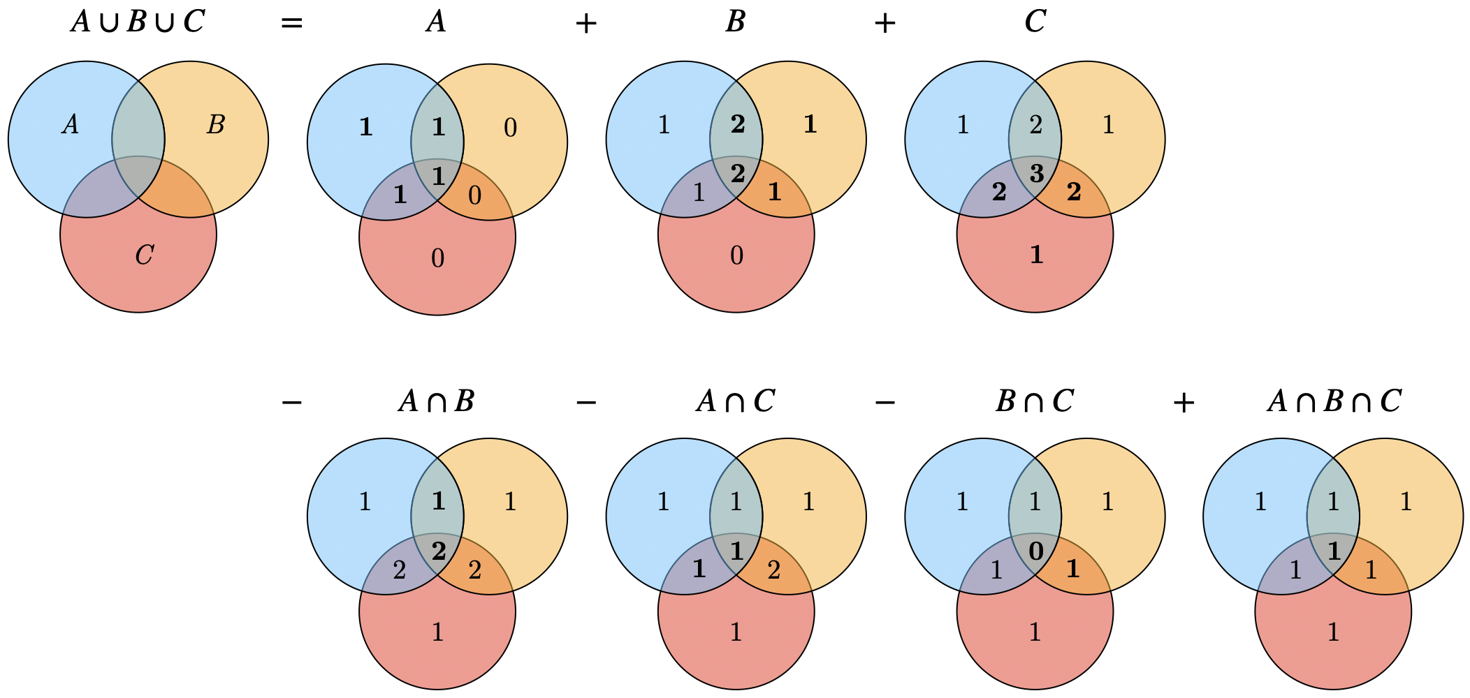
Fig. 1.12 Illustration of \(\mathbb{P}[A\cup B \cup C]\). The numbers count how many times we have added or subtracted each set in the ven diagram.

This formula generalizes for larger unions using the inclusion-exclusion rule:

(1.1)\[\begin{split}&\mathbb{P}\left[\bigcup_{i = 1}^n A_i\right]\\ =\, &\sum_{i = 1}^n \mathbb{P}[A_i] - \sum_{i < j}\mathbb{P}[A_i \cap A_j] + \sum_{i < j < k} \mathbb{P}[A_i \cap A_j \cap A_k] - \cdots + (-1)^{n+1}\mathbb{P}[A_1 \cap \cdots \cap A_n].\end{split}\]

The notation \(\sum_{i < j < k}\) means that we are summing over all indices \(i,j,k\in \{1, \dots, n\}\) such that \(i < j < k\), of which there are \({n \choose 3}\).

Fig. 1.13 Example of a winning order in Montmort’s matching game.

Fig. 1.14 Example of a losing order in Montmort’s matching game.

Example: de Montmort’s matching game.

This is Example 1.6.4 from [BH19].

This example is a bit involved, but I think it’s a great example because it ties together everything we’ve learned so far in class. I encourage you to work through it slowly!

Suppose you have a deck of \(n\) cards, with each card labeled \(1\) through \(n\). You flip the cards over one by one, saying the numbers “1”, “2”, “3”, \(\dots\) as you do so. You “win” if, at some point, the number you say aloud is the same as the number written on the card. See Figure 1.13 for an order that will cause you to win and Figure 1.14 for an order that will cause you to lose.

Question Let \(A\) be the event that you win. What is \(\mathbb{P}[A]\)?

We will work through the solution step by step.

Step 1: Define the events

Let \(A_j\) be the event that the \(j^{th}\) card in the deck is labeled \(j\). Notice that \(A\) is the event that \(A_1\) happens, or \(A_2\) happens, or \(A_3\) happens, and so on. In other words, \(A = A_1 \cup A_2 \cup \cdots \cup A_n\).

Step 2: Define the goal

Our goal will be to compute \(\mathbb{P}[A] = \mathbb{P}[A_1 \cup A_2 \cup \cdots \cup A_n]\) using the inclusion-exclusion principal from Equation (1.1).

Step 3: Compute the individual probabilities

This is the most involved step: we need to compute each of the individual probabilities from Equation (1.1).

Let’s start with \(\mathbb{P}[A_j]\), for an arbitrary \(j \in \{1, 2, \dots, n\}\). Since the deck is perfectly shuffled, all \(n\) positions are equally likely for the card labeled \(j\). Therefore, \(\mathbb{P}[A_j] = \frac{1}{n}.\)

Next, we compute \(\mathbb{P}[A_1 \cap A_2]\). This is the event that the first card in the deck is labeled 1, and the second card in the deck is labeled 2. Since all orderings of the deck are equally likely, we know that

\[\begin{equation*} \mathbb{P}[A_1 \cap A_2] = \frac{\text{# orderings where $1^{st}$ card is labeled 1 and $2^{nd}$ card is labeled 2}}{\text{# possible orderings}}. \end{equation*}\]

Starting with the denominator, we know that the number of possible orderings is \(n!\), as we saw earlier in this chapter. Next, the numerator is equal to \((n-2)!\). This is because we know the first card is labeled 1 and the second card is labeled 2, which leaves \(n-2\) remaining cards. There are \((n-2)!\) ways to order them. Therefore,

\[\begin{equation*} \mathbb{P}[A_1 \cap A_2] = \frac{(n-2)!}{n!} = \frac{(n-2)\cdot(n-3)\cdots 3 \cdot 2 \cdot 1}{n \cdot (n-1) \cdot (n-2)\cdot(n-3)\cdots 3 \cdot 2 \cdot 1} = \frac{1}{n\cdot (n-1)}. \end{equation*}\]

Similarly, \(\mathbb{P}[A_i \cap A_j] = \frac{1}{n\cdot (n-1)}\) for all \(i \not= j\). Note that there are \({n \choose 2}\) of these pair-wise intersections summed in Equation (1.1).

Generalizing this logic, we can see that for any intersection of \(k\) of these events, say \(A_1 \cap A_2 \cap \cdots \cap A_k\),

\[\begin{equation*} \mathbb{P}[A_1 \cap \cdots \cap A_k] = \frac{(n-k)!}{n!}. \end{equation*}\]

There are \({n \choose k}\) of these \(k\)-wise intersections summed in Equation (1.1).

Step 4: Plug in to compute the final answer.

Finally, we get that

\[\begin{align*}\mathbb{P}[A] &= n\cdot \frac{1}{n} - {n \choose 2}\cdot \frac{(n-2)!}{n!} + {n \choose 3} \cdot \frac{(n-3)!}{n!} - \cdots\\ &= n \cdot \frac{1}{n} - \frac{n!}{(n-2)! 2!}\cdot \frac{(n-2)!}{n!} + \frac{n!}{(n-3)! 3!}\cdot \frac{(n-3)!}{n!} - \cdots\\ &= 1 - \frac{1}{2!} + \frac{1}{3!} - \cdots \end{align*}\]

It turns out that by a Taylor expansion, \(1 - \frac{1}{2!} + \frac{1}{3!} - \cdots \approx 1 - \frac{1}{e}\) (don’t worry, I don’t expect you to remember Taylor expansions for this class), so \(\mathbb{P}[A] \approx 1 - \frac{1}{e}\). Surprisingly, this answer doesn’t depend on the number of cards \(n\). Intuitively, this is because as \(n\) grows, we have more possible matching locations but a lower probability that any one match occurs. Ultimately, this tradeoff ends up canceling out to get a final probability of \(1 - \frac{1}{e}\), independent of \(n\).