5. Continuous random variables

Up to this point, we have focused on discrete random variables, which have values that can be written down as a list. In this chapter, we will explore continuous random variables, which can assume any real value within a given interval—potentially extending infinitely, from \(-\infty\) to \(\infty\).

5.1. Probability density functions

To build intuition, recall that for a discrete RV \(X\) with PMF \(f_X(x) = \mathbb{P}[X = x]\), we can calculate the probability it falls within some interval by summing up its PMF in this interval. For example, if \(X \sim \text{Bin}(4, 0.5)\), for example, then \(\mathbb{P}[1 \leq X \leq 3] = \mathbb{P}[X = 1] + \mathbb{P}[X = 2] + \mathbb{P}[X = 3] = f_X(1) + f_X(2) + f_X(3).\)

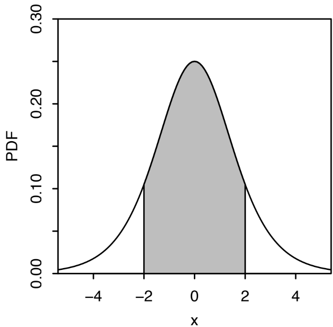
A continuous RV has a probability density function (PDF) that’s defined similarly. In particular, we say that the RV \(X\) has PDF \(f_X(x)\) if \(\mathbb{P}[a \leq X \leq b] = \int_a^b f_X(x) \, dx\). The only difference here is that instead of summing up the PMF over the discrete values, we are taking the integral over a continuous range (this intuitively makes sense since, as we learn in calculus class, an integral is a continuous version of a summation). The PDF of a continuous RV is illustrated in the following figure.

Fig. 5.1 This is Figure 5.2 from [BH19]. It illustrates the PDF of a continuous RV \(X\). To calculuate \(\mathbb{P}[-2 \leq X \leq 2]\), we compute the integral of the function between \(-2\) and \(2\), which is the shaded region.

To be a valid PDF, it must be the case that \(f_X(x) \geq 0\) and \(\int_{-\infty}^\infty f_X(x) \, dx = 1\).

It immediately follows that a continuous RV’s cumulative distribution function (CDF) is defined as \(F_X(x) = \mathbb{P}[X \leq x] = \int_{-\infty}^x f_X(t) \, dt\). Remembering the fundamental theorem of calculus, it follows that if we know a RV’s CDF, we can figure out its PDF by taking the derivative: \(f_X(x) = F'_X(x)\). The CDF also allows us to easily compute the probability \(X\) falls within an interval: \(\mathbb{P}[a < X < b] = \int_a^b f_X(x) \, dx = F_X(b) - F_X(a)\).

It’s important to understand the differences between a discrete RV’s PMF and a continuous RV’s PDF. If we evaluate the PDF of a continuous RV \(X\) at some number, say 3, it’s important to remember that \(f_X(3) \not= \mathbb{P}[X=3]\) because, by definition, \(\mathbb{P}[X = 3] = \int_3^3 f_X(x) \, dx = 0\). However, it is the case that the probability \(X\) is in some tiny interval \((3, 3 + \epsilon)\) is approximately \(f_X(3)\epsilon\):

\[\begin{equation*}\mathbb{P}\left[3 < X < 3 + \epsilon \right] = \int_{3}^{3 + \epsilon} f_X(x) \, dx \approx f_X(3)\epsilon. \end{equation*}\]

Building on the intuition that an integral is just a continuous version of a sum, we define the expected value of a continuous RV in exactly the way you would expect:

\[\begin{equation*} \mathbb{E}[X] = \int_{-\infty}^{\infty} x f_X(x) \, dx. \end{equation*}\]

Similarly, even the law of the unconscious statistician (LOTUS) carries over directly:

\[\begin{equation*} \mathbb{E}[g(X)] = \int_{-\infty}^{\infty} g(x) f_X(x) \, dx. \end{equation*}\]

In the following table, we summarize the continuous analog of the concepts we learned for discrete RVs.

Discrete	Continuous
\( X \) takes on values from a list \( x_1, x_2, \dots \)	\( X \) can be anything between \( -\infty \) and \( \infty \)
PMF \( f_X(x) = \mathbb{P}[X = x] \)	PDF \( f_X(x) \) (but \( \mathbb{P}[X = x] = 0 \))
CDF \( F_X(x) = \mathbb{P}[X \leq x] = \sum_{x_i \leq x} f_X(x_i) \)	CDF \( F_X(x) = \mathbb{P}[X \leq x] = \int_{-\infty}^x f_X(t) \, dt \)
Expectation \( \mathbb{E}[X] = \sum x f_X(x) \)	\( \mathbb{E}[X] = \int_{-\infty}^{\infty} x f_X(x) \, dx \)
LOTUS \( \mathbb{E}[g(X)] = \sum g(x) f_X(x) \)	\( \mathbb{E}[g(X)] = \int_{-\infty}^{\infty} g(x) f_X(x) \, dx \)

5.2. Uniform

For a given interval \((a, b)\), a uniform random variable represents a “completely random” point somewhere between \( a \) and \( b \). In a uniform distribution, the probability of selecting a point within any sub-interval is proportional to the length of that interval.

If we denote this random variable as \( X \sim \text{Unif}(a, b) \), then its probability density function (PDF) \( f_X(x) \) is defined as:

\[\begin{equation*} f_X(x) = \begin{cases} c & \text{if } a \leq x \leq b \\ 0 & \text{else} \end{cases} \end{equation*}\]

To determine the value of \( c \), we use the fact that the total area under the PDF over the interval \((a, b)\) must be equal to 1. This means:

\[\begin{equation*} 1 = \int_{-\infty}^{\infty} f_X(x) \, dx = \int_{-\infty}^a 0 \, dx + \int_a^b c \, dx + \int_b^{\infty} 0 \, dx = 0 + c(b - a) + 0. \end{equation*}\]

Solving for \( c \) gives:

\[\begin{equation*} c = \frac{1}{b - a}. \end{equation*}\]

Thus, for a uniform random variable \( X \) over \((a, b)\), the PDF is \( f_X(x) = \frac{1}{b - a} \) for \( a \leq x \leq b \) and 0 otherwise. For example, if \( X \sim \text{Unif}(0, 1) \), then the PDF is:

\[\begin{equation*} f_X(x) = \begin{cases} 1 & \text{if } 0 \leq x \leq 1 \\ 0 & \text{else} \end{cases} \end{equation*}\]

Meanwhile, if \( X \sim \text{Unif}\left(\frac{1}{2}, 1\right) \), then the PDF is:

\[\begin{equation*} f_X(x) = \begin{cases} \frac{1}{1 - \frac{1}{2}} = 2 & \text{if } \frac{1}{2} \leq x \leq 1 \\ 0 & \text{else} \end{cases} \end{equation*}\]

The CDF of a continuous uniform random variable \( X \) over an interval \((a, b)\) is defined as follows:

1. When \( x < a \): Since \( x \) is less than the lower bound \( a \), the probability \( \mathbb{P}[X \leq x] \) is zero. Mathematically, \(\mathbb{P}[X \leq x] = \int_{-\infty}^x 0 \, dt = 0.\)

2. When \( a \leq x \leq b \): In this case, \( x \) falls within the interval \((a, b)\), so we calculate \( \mathbb{P}[X \leq x] \) by integrating \( f_X(t) \) from \( a \) to \( x \): \(\mathbb{P}[X \leq x] = \int_a^x f_X(t) \, dt = \int_a^x \frac{1}{b - a} \, dt = \frac{x - a}{b - a}.\)

3. When \( x > b \): Here, \( x \) is greater than the upper bound \( b \), meaning \( X \) is certainly less than or equal to \( x \), so \( \mathbb{P}[X \leq x] = 1 \).

To summarize, the CDF \( F_X(x) = \mathbb{P}[X \leq x] \) for a uniform random variable \( X \sim \text{Unif}(a, b) \) is:

\[\begin{equation*} F_X(x) = \begin{cases} 0 & \text{if } x < a \\ \frac{x - a}{b - a} & \text{if } a \leq x \leq b \\ 1 & \text{if } x > b. \end{cases} \end{equation*}\]

For example, if \( X \sim \text{Unif}(0, 1) \), the CDF becomes:

\[\begin{equation*} F_X(x) = \begin{cases} 0 & \text{if } x < 0 \\ x & \text{if } 0 \leq x \leq 1 \\ 1 & \text{if } x > 1. \end{cases} \end{equation*}\]

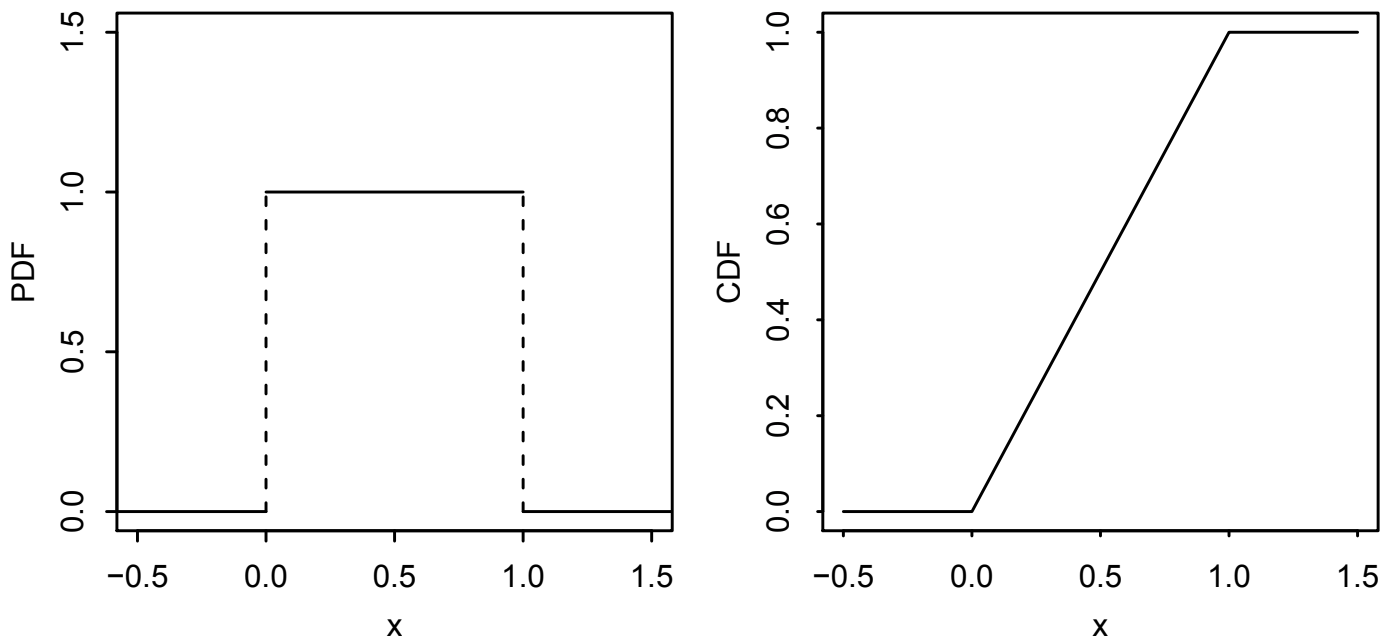
The following figure illustrates the PDF and CDF of the \(\text{Unif}(0, 1) \) distribution.

Fig. 5.2 This is Figure 5.6 from [BH19]. It illustrates the PDF and CDF of the \(\text{Unif}(0, 1) \) distribution.

5.2.1. Expectation of \( X \)

The expectation of \( X \) is given by:

\[\begin{equation*} \mathbb{E}[X] = \int_{-\infty}^{\infty} x f_X(x) \, dx = \int_a^b \frac{x}{b - a} \, dx. \end{equation*}\]

Evaluating this integral, we find:

\[\begin{equation*} \mathbb{E}[X] = \left. \frac{x^2}{2(b - a)} \right|_a^b = \frac{b^2 - a^2}{2(b - a)} = \frac{a + b}{2}. \end{equation*}\]

For a uniform random variable \( X \sim \text{Unif}(0, 1) \), this yields \( \mathbb{E}[X] = \frac{0 + 1}{2} = \frac{1}{2} \).

5.2.2. Variance of \( X \)

The variance of \( X \) is \( \text{Var}(X) = \mathbb{E}[X^2] - \mathbb{E}[X]^2 \). First, we calculate \( \mathbb{E}[X^2] \) using LOTUS:

\[\begin{equation*} \mathbb{E}[X^2] = \int_a^b x^2 f_X(x) \, dx = \left. \frac{x^3}{3(b - a)} \right|_a^b = \frac{b^3 - a^3}{3(b - a)}. \end{equation*}\]

Then, the variance becomes:

\[\begin{equation*} \text{Var}(X) = \frac{b^3 - a^3}{3(b - a)} - \left(\frac{a + b}{2}\right)^2 = \frac{(b - a)^2}{12}. \end{equation*}\]

5.3. Normal

Bell curves are remarkably prevalent in the world around us. The normal distribution is commonly used to model events and variables that exhibit this characteristic “bell curve” shape.

Standard normal distribution

A standard normal random variable \( Z \) has the probability density function (PDF):

\[\begin{equation*} \varphi(t) = \frac{1}{\sqrt{2\pi}}e^{-t^2/2}. \end{equation*}\]

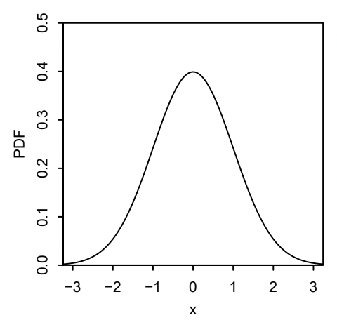
This distribution is so famous that we use the special notation \(\varphi(t)\) to denote its PDF. See Figure 5.3 for an illustration.

We use the notation \( Z \sim N(0,1) \) to represent this RV’s distribution. In this case, the parameters \(0\) and \(1\) indicate that \( Z \) has a mean of \( 0 \) and a variance of \( 1 \).

Fig. 5.3 This is Figure 5.11 from [BH19], illustrating the PDF of the standard normal distribution.

To find the probability that \( Z \) lies between two values \( a \) and \( b \), we compute:

\[\begin{equation*} \mathbb{P}[a \leq Z \leq b] = \int_a^b \varphi(t) \, dt. \end{equation*}\]

The cumulative distribution function (CDF) of \( Z \), represented as \( \Phi(t) \) (which is the capital letter version of the Greek letter \(\varphi\)), gives the probability that \( Z \) is less than or equal to a given value \( t \):

\[\begin{equation*} \Phi(t) = \mathbb{P}[Z \leq t] = \frac{1}{\sqrt{2\pi}}\int_{-\infty}^t e^{-y^2/2} \, dy. \end{equation*}\]

The expected value of \( Z \), \( \mathbb{E}[Z] \), is \( 0 \), calculated by

\[\begin{equation*} \mathbb{E}[Z] = \int_{-\infty}^{\infty} t \varphi(t) \, dt = 0, \end{equation*}\]

and the variance of \( Z \), \( \text{Var}(Z) \), is \( 1 \). See the textbook for the derivation of these quantities.

Normal distribution

If we have a random variable \( Z \sim N(0,1) \), then the transformation \( X = \mu + \sigma Z \) yields a new normal distribution with mean \( \mu \) and variance \( \sigma^2 \). We denote this as \( X \sim N(\mu, \sigma^2) \).

Intuitively, by applying the transformation \( X = \mu + \sigma Z \), we are shifting the peak of the bell curve in Figure 5.3 over from \(0\) to \(\mu\), and we are squashing or stretching the bell curve by multiplying \(Z\) by \(\sigma\).

To verify that the expected value of \( X \sim N(\mu, \sigma^2) \) is indeed \(\mu\), we can use linearity of expectation:

\[\begin{equation*} \mathbb{E}[X] = \mathbb{E}[\mu + \sigma Z] = \mu + \sigma \mathbb{E}[Z] = \mu. \end{equation*}\]

Similarly, the variance of \( X \), \( \text{Var}(X) \), is:

\[\begin{equation*} \text{Var}(X) = \sigma^2 \text{Var}(Z) = \sigma^2. \end{equation*}\]

The cumulative distribution function (CDF) of \( X \) provides the probability that \( X \) is less than or equal to a value \( t \). This is calculated by standardizing \( X \) (subtracting \( \mu \) and dividing by \( \sigma \)) to relate it to \( Z \):

\[\begin{equation*} \mathbb{P}[X \leq t] = \mathbb{P}\left[\frac{X - \mu}{\sigma} \leq \frac{t - \mu}{\sigma}\right] = \mathbb{P}\left[Z \leq \frac{t - \mu}{\sigma}\right] = \Phi\left(\frac{t - \mu}{\sigma}\right), \end{equation*}\]

where \( \Phi \) is the CDF of the standard normal distribution. Finally, the probability density function (PDF) of \( X \), obtained using the chain rule for transformations, is:

\[\begin{equation*} f_X(t) = \frac{1}{\sigma \sqrt{2\pi}} \exp\left(-\frac{(t - \mu)^2}{2\sigma^2}\right). \end{equation*}\]

Although the PDF and CDF of the normal distribution are unweildy and difficult to work with, there are simple heuristics we can use the work with this random variable. In particular, the 68-95-99.7 rule is a useful guideline for interpreting probabilities in a normal distribution. For \( X \sim N(\mu, \sigma^2) \), this rule states:

• Approximately 68% of the values lie within one standard deviation of the mean, so \(\mathbb{P}[|X - \mu| < \sigma] \approx 0.68\).

• Roughly 95% of the values are within two standard deviations, meaning \(\mathbb{P}[|X - \mu| < 2\sigma] \approx 0.95\).

• Nearly all values, about 99.7%, fall within three standard deviations, or \(\mathbb{P}[|X - \mu| < 3\sigma] \approx 0.997\).

Example: Stock prices

To illustrate this, suppose you are forecasting a stock price that follows a normal distribution with a mean \(\mu = 100\) and a standard deviation \(\sigma = 3\). Your prediction for the stock price is exactly \(100\). You’ll receive a bonus if your forecast error—meaning the difference between the actual and predicted price—is smaller than \(6\). According to the 68-95-99.7 rule, the probability that the actual stock price will fall within \(6\) units of your prediction (i.e., within two standard deviations) is approximately 95%. Therefore, \(\mathbb{P}[\text{bonus}] = 0.95\).

5.4. Exponential

The exponential distribution is commonly used to model the time interval between consecutive events. This distribution is particularly useful in scenarios where events occur randomly and independently over time. Examples of processes that can be modeled by an exponential distribution include:

• The arrival of emergencies at a hospital,

• The occurrence of catastrophic events, such as a sudden stock market crash,

• Equipment breakdowns in manufacturing or industrial settings.

If a random variable \( X \) follows an exponential distribution with a rate parameter \( \lambda \), then its probability density function (PDF) is given by:

\[\begin{equation*} f_X(t) = \lambda e^{-\lambda t}, \quad t > 0. \end{equation*}\]

The cumulative distribution function (CDF) of \( X \) provides the probability that \( X \) will occur within a given time \( t \). It is calculated as follows:

\[\begin{equation*} F_X(t) = \int_0^t \lambda e^{-\lambda y} \, dy = -e^{-\lambda y} \Big|_0^t = 1 - e^{-\lambda t} = \mathbb{P}[X < t]. \end{equation*}\]

The expected value or mean of \( X \), \( \mathbb{E}[X] \), is \( \frac{1}{\lambda} \), which represents the average time between events. The variance of \( X \), \( \text{Var}(X) \), is \( \frac{1}{\lambda^2} \), indicating the spread or variability of the time intervals between events.

The exponential distribution is unique in that it possesses a property known as memorylessness. As [BH19] puts it, this property says that “even if you’ve waited for hours or days without success, the success isn’t any more likely to arrive soon. In fact, you might as well have just started waiting 10 seconds ago.” Mathematically, for a random variable \( X \) that follows an exponential distribution, this memoryless property can be expressed as:

\[\begin{equation*} \mathbb{P}[X \geq s + t \mid X \geq s] = \mathbb{P}[X \geq t]. \end{equation*}\]

This equation states that the probability of waiting at least an additional time \( t \), given that at least \( s \) units of time have already passed, is simply the probability of waiting at least \( t \) from the beginning. We can derive this as follows:

\[\begin{equation*} \mathbb{P}[X \geq s + t \mid X \geq s] = \frac{\mathbb{P}[X \geq s + t \text{ and }X \geq s]}{\mathbb{P}[X \geq s]} = \frac{\mathbb{P}[X \geq s + t]}{\mathbb{P}[X \geq s]} = \frac{e^{-\lambda(s + t)}}{e^{-\lambda s}} = e^{-\lambda t} = \mathbb{P}[X \geq t]. \end{equation*}\]

Interestingly, if \( X \) is a positive, memoryless, and continuous random variable, then \( X \) must follow an exponential distribution.

Example: Hospital bed waiting time

Suppose an emergency room (ER) has 10 beds, where the time a patient time spends occupying a bed follows an exponential distribution. Specifically, the time in the \(i\)-th bed is modeled by an exponential distribution with rate parameter \(\lambda_i\). Suppose Alice arrives at the ER at midnight. All 10 beds are currently occupied, but Alice is next in line to be assigned a bed.

Question: What is the probability that Alice is still waiting for an available bed at 12:30 (30 minutes after her arrival)?

Step 1: Define the Random Variables

Let \( X_i \) represent the number of minutes after midnight until the \(i\)-th bed becomes available, for \( i = 1, 2, \dots, 10 \). By the memoryless property of the exponential distribution, each \( X_i \sim \text{Expo}(\lambda_i) \), meaning it does not matter how long each patient has already been in their bed; the remaining time is still governed by an exponential distribution.

Step 2: Compute the Probability

We want to determine the probability that Alice needs to wait at least 30 minutes, or mathematically, \( \mathbb{P}[\min\{X_1, X_2, \dots, X_{10}\} > 30] \). This probability can be computed as follows:

\[\begin{equation*} \mathbb{P}[\min\{X_1, X_2, \dots, X_{10}\} > 30] = \mathbb{P}[X_1 > 30 \text{ and } X_2 > 30 \text{ and } \dots X_{10} > 30]. \end{equation*}\]

Since each \( X_i \) is an independent exponential random variable:

\[\begin{equation*} \mathbb{P}[X_1 > 30] \cdots \mathbb{P}[X_{10} > 30] = \left(1 - \mathbb{P}[X_1 < 30]\right) \cdots \left(1 - \mathbb{P}[X_{10} < 30]\right). \end{equation*}\]

For each bed \( i \), \( \mathbb{P}[X_i > 30] = e^{-30 \lambda_i} \), so we get:

\[\begin{equation*} \mathbb{P}[\min\{X_1, X_2, \dots, X_{10}\} > 30] = e^{-30 \lambda_1} \cdots e^{-30 \lambda_{10}} = e^{-30(\lambda_1 + \cdots + \lambda_{10})}. \end{equation*}\]

Insight: The minimum of these waiting times, \( \min\{X_1, X_2, \dots, X_{10}\} \), follows an exponential distribution with a combined rate parameter \( \lambda_1 + \cdots + \lambda_{10} \).

5.5. Poisson processes

Poisson processes are one of the most useful models of events occurring randomly over time.

Poisson process

A sequence of arrivals in continuous time is called a Poisson process with rate \( \lambda \) if it satisfies the following conditions:

• The number of arrivals, denoted \( X \), within an interval of length \( t \) is a Poisson random variable with parameter \( \lambda t \). This means that the probability of observing exactly \( k \) arrivals in that interval is given by \(\mathbb{P}[X = k] = \frac{e^{-\lambda t} (\lambda t)^k}{k!}.\)

• The number of arrivals in disjoint time intervals are independent of each other. For instance, the counts of arrivals in the intervals \( (0, 10) \), \( [10, 12) \), and \( [15, \infty) \) are mutually independent.

Example: Arrivals at SFO

Suppose people at San Francisco International Airport according to a Poisson process with a rate of \( \lambda = 50 \) arrivals per minute. This means, for example that:

• Since one minute is an interval of length 1, the number of people expected to arrive in one minute follows a Poisson distribution with parameter \( 50 \), denoted as \( \text{Pois}\left(50\right) \).

• For a 30-second interval (half a minute), the number of people arriving in that time frame follows the \( \text{Pois}\left(\frac{50}{2}\right) \) distribution.

Question: Let \(T_1\) be the time the first customer arrives (starting from when SFO opens in the morning). What is the distribution of \(T_1\)?

Step 1: Define the random variables. Since we are working with a Poisson process, we know that if \( N_t \) is the number of customers arriving by time \( t \), then \( N_t \sim \text{Pois}(50t) \).

Step 2: Determine the relationship between the random variables. We want to understand the relationship between \(T_1\) and \(N_t\). Starting with an example, we know that the event \( T_1 > \frac{1}{2} \) (no arrival in the first half minute) occurs if and only if \( N_{1/2} = 0 \), meaning no arrivals have occurred by time \( \frac{1}{2} \) (measured in minutes). More generally, \( T_1 > t \) if and only if \( N_t = 0 \), indicating that no arrivals have occurred by time \( t \).

Step 3: Calculate the CDF of \( T_1 \). The probability \( \mathbb{P}[T_1 > t] \) is the probability of zero arrivals in the interval \( [0, t] \), calculated as:

\[\begin{equation*} \mathbb{P}[T_1 > t] = \mathbb{P}[N_t = 0] = \frac{e^{-\lambda t}\lambda^0}{0!} = e^{-50t}. \end{equation*}\]

Therefore, the cumulative distribution function (CDF) of \( T_1 \) is:

\[\begin{equation*} \mathbb{P}[T_1 < t] = 1 - \mathbb{P}[T_1 > t] = 1 - e^{-50t}. \end{equation*}\]

This is exactly the CDF of the exponential distribution with parameter \(\lambda = 50\), indicating that \( T_1 \sim \text{Expo}\left(50\right) \).

Similarly, let \( T_2 \) is the time of the second arrival, and note that the interval \( (T_1, T_2] \) is disjoint from \( [0, T_1] \). Thus, the waiting time between the first and second arrivals, \( T_2 - T_1 \), also follows an exponential distribution with rate \( 50 \).

General rule

In general, if a sequence of arrivals is a Poisson process with rate \(\lambda\), then the time between each arrival has the Expo\((\lambda)\) distribution.