6. Joint distributions

Until now, whenever we have analyzed multiple random variables in a single problem, we have assumed they were independent—that is, information about one random variable gave us no insight into the others. While independence is a useful assumption for simplifying calculations, most random variables are not independent. In this chapter, we will develop tools to jointly analyze dependent random variables.

6.1. Joint, marginal, and conditional

6.1.1. Discrete

Let \( X \) and \( Y \) be two discrete random variables.

Joint cumulative distribution function (CDF)

The joint CDF of \( X \) and \( Y \), denoted \( F_{X,Y}(x,y) \), is defined as the probability that \( X \leq x \) and \( Y \leq y \), or \( F_{X,Y}(x,y) = \mathbb{P}[X \leq x, Y \leq y] \).

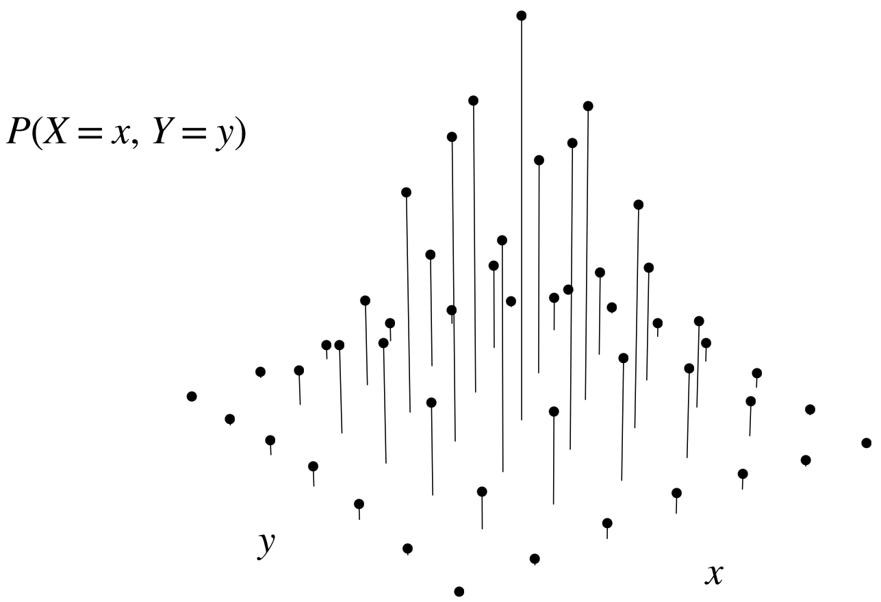
Fig. 6.1 This is Figure 7.1 from [BH19]. It illustrates the joint PMF of two RVs \(X\) and \(Y\).

Joint probability mass function (PMF)

The joint PMF of \( X \) and \( Y \), denoted \( f_{X,Y}(x,y) \), is the probability that \( X = x \) and \( Y = y \), or \( f_{X,Y}(x,y) = \mathbb{P}[X = x, Y = y] \). See Figure 6.1 for an illustration.

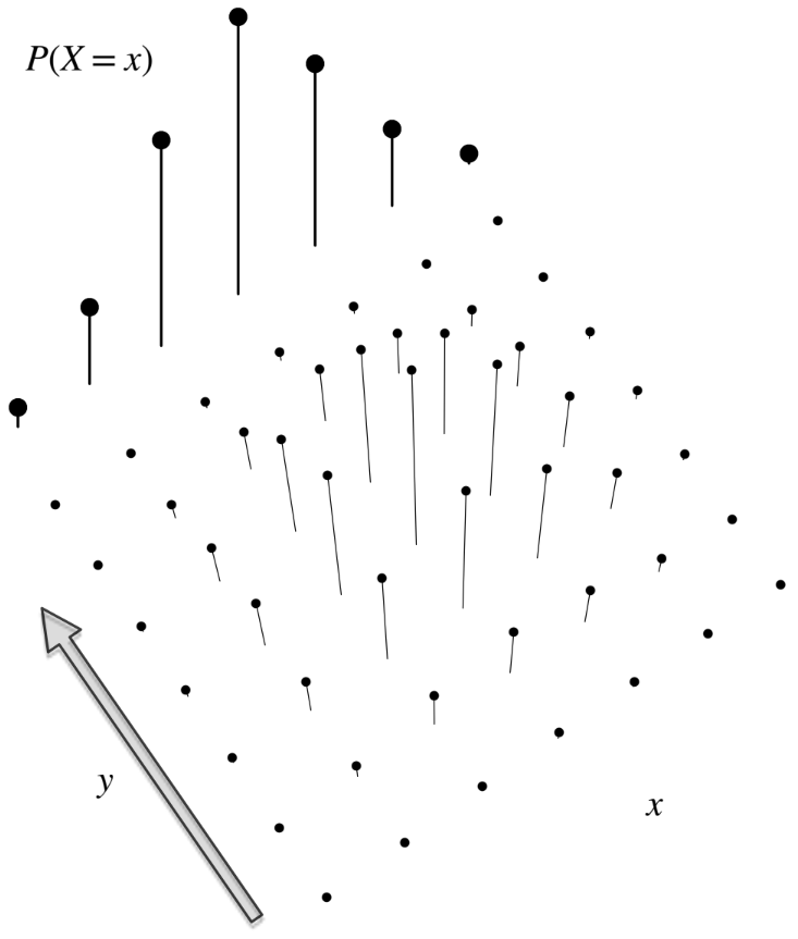
Fig. 6.2 This is Figure 7.2 from [BH19]. It is a bird’s-eye view of the PMF in Figure 6.1. As [BH19] states, the marginal PMF \(f_X(x)\) is obtained by summing over the joint PMF in the \(y\)-direction.

Marginal PMF

We obtain the marginal PMF of \( X \), \( f_X(x) = \mathbb{P}[X = x] \), via the law of total probability: we sum over the joint probabilities over all possible values of \( Y \), so

\[\begin{equation*} f_X(x) = \mathbb{P}[X = x] = \sum_y \mathbb{P}[X = x, Y = y] = \sum_y f_{X,Y}(x,y). \end{equation*}\]

The marginal PMF of \(Y\), \(f_Y(y)\), is defined symmetrically. See Figure 6.2 for an illustration.

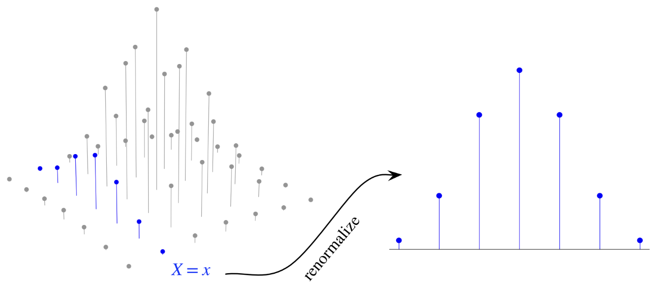
Fig. 6.3 This is Figure 7.3 from [BH19]. To obtain the conditional PMF \(\mathbb{P}[Y = y \mid X = x]\), we renormalize the slice of the joint PMF that corresponds to the event that \(X = x\).

Conditional PMF

The conditional PMF of \( Y \) given \( X = x \), \( \mathbb{P}[Y = y \mid X = x] \), represents the probability that \( Y = y \) given that \( X = x \). It is calculated using the definition of conditional probability

\[\begin{equation*} \mathbb{P}[Y = y \mid X = x] = \frac{\mathbb{P}[X = x, Y = y]}{\mathbb{P}[X = x]}, \end{equation*}\]

assuming \( \mathbb{P}[X = x] > 0.\) The conditional PMF of \(X\) given \(Y = y\) is defined symmetrically. See Figure 6.3 for an illustration.

Table 6.1 Joint PMF of \( X \) and \( Y \) for the following basketball free throw example.

	\( Y = 1 \)	\( Y = 0 \)
\( X = 1 \)	\( f_{X,Y}(1,1) = \mathbb{P}[X = 1, Y = 1] = \frac{5}{100} \)	\( f_{X,Y}(1,0) = \frac{20}{100} \)
\( X = 0 \)	\( f_{X,Y}(0,1) = \frac{3}{100} \)	\( f_{X,Y}(0,0) = \frac{72}{100} \)

Example: Basketball free throws

Suppose we want to analyze the likelihood of a player making two consecutive free throws in a game. Let \( X \) be an indicator variable representing whether a player makes the first free throw (1 if they make it, 0 if they miss), and \( Y \) is an indicator variable representing whether they make the second free throw.

The joint PMF of \(X\) and \(Y\) is given in Table 6.1.

The marginal PMF of \(X\) is \(f_X(0) = \mathbb{P}[X = 0] = f_{X,Y}(0,0) + f_{X,Y}(0,1) = \frac{25}{100}\) and \(f_X(1) = \mathbb{P}[X = 1] = f_{X,Y}(1,0) + f_{X,Y}(1,1) = \frac{75}{100}\). Similarly, the marginal PMF of \(Y\) is \(f_Y(0) = f_{X,Y}(0,0) + f_{X,Y}(1,0) = \frac{8}{100}\) and \(f_Y(1) = f_{X,Y}(0,1) + f_{X,Y}(1,1) = \frac{92}{100}\).

Finally, the conditional PMF of \(X\) given \(Y = 0\), for example, is \(\mathbb{P}[X = 0 \mid Y = 0] = \frac{f_{X,Y}(0,0)}{f_Y(0)} = \frac{5/100}{8/100} = \frac{5}{8}\) and \(\mathbb{P}[X = 1 \mid Y = 0] = 1- \frac{5}{8} = \frac{3}{8}.\)

Independence

Two random variables \( X \) and \( Y \) are said to be independent if their joint cumulative distribution function (CDF) \( F_{X,Y}(x,y) \) can be expressed as the product of their individual CDFs, \( F_X(x) \) and \( F_Y(y) \), for all values of \( x \) and \( y \). In other words, \( X \) and \( Y \) are independent if \( F_{X,Y}(x,y) = F_X(x)F_Y(y) \) holds for all possible pairs of values.

An equivalent condition for independence is that the joint probability mass function (PMF) \( f_{X,Y}(x,y) \) can be factored as the product of the marginal PMFs of \( X \) and \( Y \), i.e., \( f_{X,Y}(x,y) = f_X(x)f_Y(y) \).

Table 6.2 Joint PMF for the following coin flip example

	\( Y = 0 \)	\( Y = 1 \)
\( X = 0 \)	\( f_{X,Y}(0,0) = \mathbb{P}[X = 0, Y= 0] = 0 \)	\( f_{X,Y}(0,1) =\mathbb{P}[X = 0, Y = 1] = \mathbb{P}[X = 0] = \frac{1}{4} \)
\( X = 1 \)	\( f_{X,Y}(1,0) =\mathbb{P}[X = 1, Y= 0] = \mathbb{P}[X = 1] = \frac{1}{2} \)	\( f_{X,Y}(1,1) =0 \)
\( X = 2 \)	\( f_{X,Y}(2,0) =0 \)	\( f_{X,Y}(2,1) =\frac{1}{4} \)

Example: Coin flips

Suppose a fair coin is flipped twice. Let the random variable \( X \) represent the number of heads obtained in the two flips. Define another random variable, \( Y \), such that \( Y = 1 \) if both tosses landed the same way (either both heads or both tails), and \( Y = 0 \) otherwise.

Question 1: What is the joint probability mass function (PMF) of \( X \) and \( Y \)?

The joint PMF of \( X \) and \( Y \) is given in Table 6.2.

Question 2: What is the marginal PMF of \( X \)?

The marginal PMF of \( X \), representing the probability distribution of the number of heads, is calculated as follows:

• \( f_X(0) = \mathbb{P}[X = 0] = \mathbb{P}[X = 0, Y = 0] + \mathbb{P}[X = 0, Y = 1] = \frac{1}{4} \)

• \( f_X(1) = \mathbb{P}[X = 1, Y = 0] + \mathbb{P}[X = 1, Y = 1] = \frac{1}{2} \)

• \( f_X(2) = \frac{1}{4} \)

Question 3: What is the marginal PMF of \( Y \)?

The marginal PMF of \( Y \), representing the probability of the tosses landing the same way or not, is calculated as follows:

• \( f_Y(0) = \mathbb{P}[Y = 0] = \mathbb{P}[X = 0, Y = 0] + \mathbb{P}[X = 1, Y = 0] + \mathbb{P}[X = 2, Y = 0] = \frac{1}{2} \)

• \( f_Y(1) = \frac{1}{2} \)

Question 4: Are \( X \) and \( Y \) independent?

No, \( X \) and \( Y \) are not independent. For example, the joint probability \( f_{X,Y}(0,0) = 0 \) does not equal the product of the marginals \( f_X(0)f_Y(0) = \frac{1}{4} \cdot \frac{1}{2} = \frac{1}{8} \).

6.1.2. Continuous

Next, let \(X\) and \(Y\) be two continuous RVs. In this case, the definition of the joint CDF remains the same:

Joint cumulative distribution function (CDF)

The joint CDF of \( X \) and \( Y \), denoted \( F_{X,Y}(x,y) \), represents the probability that \( X \leq x \) and \( Y \leq y \), or \( F_{X,Y}(x,y) = \mathbb{P}[X \leq x, Y \leq y] \).

Recall that in the case of a single continuous RV, we obtain the PDF by taking the derivative of the CDF. The same holds true when working with joint continuous RVs, except we must take the derivate in terms of \(x\) and \(y\).

Joint probability density function (PDF)

The joint PDF of \( X \) and \( Y \), denoted \( f_{X,Y}(x,y) \), is obtained by taking the second partial derivative of the joint CDF with respect to both \( x \) and \( y \). In other words, \( f_{X,Y}(x,y) = \frac{\partial^2}{\partial x \partial y}F_{X,Y}(x,y) \).

Marginal PMF

The marginal PDF of \( X \), denoted \( f_X(x) \), is obtained by integrating the joint PDF over all values of \( Y \). This is expressed as \( f_X(x) = \int_{-\infty}^{\infty} f_{X,Y}(x,y) \, dy \).

Example: Uniform distribution over a square

Suppose \( (X, Y) \) is a completely random point chosen uniformly from within the square region \( \{(x,y): x, y \in [0,1]\} \) in the plane. This means that any point within the square is equally likely to be chosen.

The joint probability density function (PDF) of \( X \) and \( Y \), \( f_{X,Y}(x,y) \), is defined as follows:

\[\begin{equation*}f_{X,Y}(x,y) = \begin{cases}1 &\text{if }(x,y) \in [0,1] \times [0,1]\\ 0 &\text{else.}\end{cases}\end{equation*}\]

To find the marginal PDF of \( X \), denoted \( f_X(x) \), we integrate \( f_{X,Y}(x,y) \) over all possible values of \( y \):

\[\begin{equation*} f_X(x) = \int_{-\infty}^{\infty} f_{X,Y}(x,y) \, dy = \int_{-\infty}^0 0 \, dy + \int_0^1 1 \, dy + \int_1^{\infty} 0 \, dy = y \Big|_{0}^1 = 1. \end{equation*}\]

This result implies that \( X \) follows a uniform distribution on the interval \( [0,1] \), or \( X \sim \text{Unif}(0,1) \).

Since the joint PDF \( f_{X,Y}(x,y) \) can be factored as the product of the marginal PDFs of \( X \) and \( Y \) for all \( x, y \in [0,1] \times [0,1] \), i.e., \( f_{X,Y}(x,y) = 1 = f_X(x) f_Y(y) \), we conclude that \( X \) and \( Y \) are independent.

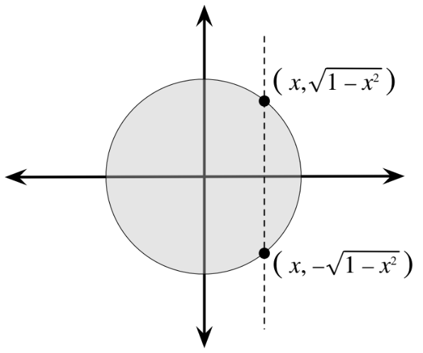
Fig. 6.4 This is Figure 7.6 from [BH19]. For a fixed \(x \in [-1,1]\), \((x,y)\) is in the unit circle centered at the origin if \(x^2 + y^2 \leq 1\), or in other words, if \(-\sqrt{1 - x^2} \leq y \leq \sqrt{1 - x^2}\).

Example: Uniform distribution over a circle

Suppose \( (X, Y) \) is a completely random point chosen uniformly from within a circle of radius 1, centered at the origin. This region can be described as \( \{(x, y) : x^2 + y^2 \leq 1\} \). Any point within this circle is equally likely to be chosen.

The joint probability density function (PDF) of \( X \) and \( Y \), denoted \( f_{X,Y}(x, y) \), is defined as follows:

\[\begin{equation*}f_{X,Y}(x,y) = \begin{cases} \frac{1}{\pi} & \text{if }x^2 + y^2\leq 1\\ 0 &\text{else}\end{cases}\end{equation*}\]

(understanding why the PDF is \(\frac{1}{\pi}\) inside the circle requires comfort with multi-variable integration, so you may take this as given—don’t worry if you don’t know how we arrived at \(\frac{1}{\pi}\)).

To find the marginal PDF of \( X \), denoted \( f_X(x) \), we integrate \( f_{X,Y}(x, y) \) over all possible values of \( y \):

\[\begin{equation*} f_X(x) = \int_{-\infty}^{\infty} f_{X,Y}(x, y) \, dy. \end{equation*}\]

We know that \(f_{X,Y}(x, y) = \frac{1}{\pi}\) so long as \((x,y)\) is in the circle of radius 1, centered at the origin, or in other words, so long as \(x^2 + y^2\leq 1\). Looking at Fig. 6.4, we can see that for a specific choice of \(x \in [-1,1]\), \(f_{X,Y}(x, y) = \frac{1}{\pi}\) so long as \(-\sqrt{1 - x^2} \leq y \leq \sqrt{1 - x^2}\). Otherwise, \(f_{X,Y}(x, y) = 0\). Therefore, for \(x \in [-1,1]\),

\[\begin{equation*} f_X(x) = \int_{-\infty}^{-\sqrt{1 - x^2}} 0 \, dy + \int_{-\sqrt{1 - x^2}}^{\sqrt{1 - x^2}} \frac{1}{\pi} \, dy + \int_{\sqrt{1 - x^2}}^{\infty} 0 \, dy = \left. \frac{y}{\pi} \right|_{-\sqrt{1 - x^2}}^{\sqrt{1 - x^2}} = \frac{2}{\pi} \sqrt{1 - x^2}. \end{equation*}\]

For \(x \not\in [-1,1]\), \(f_X(x) = 0\).

This result shows that \( X \) does not follow a uniform distribution, as \( f_X(x) \) depends on \( x \) in a non-constant way.

Moreover, \( X \) and \( Y \) are not independent. For example, \( f_{X,Y}(0.9, 0.9) = 0 \), because the point \( (0.9, 0.9) \) lies outside the circle (as \( 0.9^2 + 0.9^2 > 1 \)), even though both \( f_X(0.9) \) and \( f_Y(0.9) \) are non-zero. This demonstrates that the joint probability does not equal the product of the marginals, confirming that \( X \) and \( Y \) are dependent.

6.1.3. Hybrid

Example: Injury recovery time

Suppose an athlete has sustained an injury, but it is unclear whether the injury is minor or major.

• If the injury is minor, the time it takes to heal follows an exponential distribution with rate \( \lambda_0 \) (so the expected healing time is \( \frac{1}{\lambda_0} \)).

• If the injury is major, the healing time follows an exponential distribution with rate \( \lambda_1 \) (with expected healing time \( \frac{1}{\lambda_1} \)).

• We assume that \( \lambda_0 > \lambda_1 \), meaning that minor injuries generally heal faster than major ones.

The injury is major with probability \( p_1 \) and as minor with probability \( p_0 = 1 - p_1 \). Let \( I \) be an indicator random variable, where \( I = 1 \) if the injury is major and \( I = 0 \) if it is minor. Let \( T \) represent the time it takes for the injury to heal.

Question: What is the marginal cumulative distribution function (CDF) of \( T \)?

The marginal CDF of \( T \), denoted \( F_T(t) \), can be computed as follows:

\[\begin{equation*} F_T(t) = \mathbb{P}[T \leq t] = \mathbb{P}[T \leq t \mid I = 0] \cdot \mathbb{P}[I = 0] + \mathbb{P}[T \leq t \mid I = 1] \cdot \mathbb{P}[I = 1]. \end{equation*}\]

Substituting the expressions for each conditional probability, we get:

\[\begin{equation*} F_T(t) = \left(1 - e^{-\lambda_0 t}\right)p_0 + \left(1 - e^{-\lambda_1 t}\right)p_1 = 1 - p_0 e^{-\lambda_0 t} - p_1 e^{-\lambda_1 t}. \end{equation*}\]

Question: What is the marginal probability density function (PDF) of \( T \)?

The marginal PDF of \( T \), denoted \( f_T(t) \), is the derivative of \( F_T(t) \) with respect to \( t \):

\[\begin{equation*} f_T(t) = \frac{d}{dt} F_T(t) = p_0 \lambda_0 e^{-\lambda_0 t} + p_1 \lambda_1 e^{-\lambda_1 t}. \end{equation*}\]

6.2. 2D LOTUS

The law of the unconscious statistician extends naturally to joint random variables. We will only state it here for discrete RVs (the definition for continuous RVs involves multi-variable integration, which we do not assume knowledge of in this class).

2D Law of the unconscious statistician (LOTUS)

Let \( g: \mathbb{R}^2 \to \mathbb{R} \) be a function. When \( X \) and \( Y \) are discrete random variables, the expected value of \( g(X, Y) \), denoted \( \mathbb{E}[g(X, Y)] \), is calculated as

\[\begin{equation*} \mathbb{E}[g(X, Y)] = \sum_x \sum_y g(x, y) \cdot \mathbb{P}[X = x, Y = y]. \end{equation*}\]

Table 6.3 Joint PMF of \( X \) and \( Y \) for shots and goals in soccer

	\( X = 1 \)	\( X = 2 \)
\( Y = 0 \)	\( \frac{3}{10} \)	\( \frac{2}{10} \)
\( Y = 1 \)	\( \frac{1}{10} \)	\( \frac{3}{10} \)
\( Y = 2 \)	\( 0 \)	\( \frac{1}{10} \)

Example: Shots per goal in soccer

In the first 15 minutes of a soccer match, a team will make between 1 and 2 shots on goal. Let \( X \) represent the number of shots taken and \( Y \) represent the number of goals scored. The joint probability distribution of \( X \) and \( Y \) is given by Table 6.3.

Question: What is the expected number of goals per shot?

To find this, we calculate \( \mathbb{E}\left[\frac{Y}{X}\right] \) as follows:

\[\begin{equation*} \mathbb{E}\left[\frac{Y}{X}\right] = \frac{0}{1} \cdot \frac{3}{10} + \frac{1}{1} \cdot \frac{1}{10} + \frac{0}{2} \cdot \frac{2}{10} + \frac{1}{2} \cdot \frac{3}{10} + \frac{2}{2} \cdot \frac{1}{10} = \frac{7}{20}. \end{equation*}\]

Thus, the expected number of goals per shot is \( \frac{7}{20} \).

6.3. Covariance and correlation

Covariance provides insight into the relationship between two variables, specifically in terms of how they vary together. Unlike variance, which measures the variability of a single variable, covariance captures how two variables move in relation to each other.

Covariance

The covariance of two random variables \(X\) and \(Y\), denoted as \(\text{Cov}(X, Y)\), is given by

\[\begin{equation*} \text{Cov}(X, Y) = \mathbb{E}[(X - \mathbb{E}[X])(Y - \mathbb{E}[Y])] = \mathbb{E}[XY] - \mathbb{E}[X]\mathbb{E}[Y]. \end{equation*}\]

When \(X\) and \(Y\) tend to move in the same direction (both increasing or both decreasing together), the covariance \(\text{Cov}(X, Y)\) will be positive.

Conversely, if \(X\) and \(Y\) tend to move in opposite directions (one increases while the other decreases), then \(\text{Cov}(X, Y)\) will be negative.

If \(X\) and \(Y\) are independent, they are uncorrelated, meaning \(\mathbb{E}[XY] = \mathbb{E}[X]\mathbb{E}[Y]\), which implies \(\text{Cov}(X, Y) = 0\). However, it is worth noting that \(\text{Cov}(X, Y) = 0\) does not necessarily imply that \(X\) and \(Y\) are independent; two variables can have zero covariance and still be dependent in a non-linear way.

The covariance function has several key properties:

1. The covariance of a variable with itself, \(\text{Cov}(X, X)\), is simply the variance of \(X\), written as \(\text{Var}(X)\).

2. Covariance is symmetric, meaning \(\text{Cov}(X, Y) = \text{Cov}(Y, X)\).

3. For the variance of the sum of multiple variables \(X_1, X_2, \dots, X_n\), we have

   \[\begin{equation*} \text{Var}(X_1 + X_2 + \cdots + X_n) = \text{Var}(X_1) + \cdots + \text{Var}(X_n) + 2\sum_{i < j} \text{Cov}(X_i, X_j). \end{equation*}\]

Example: Hypergeometric variance

Remember that the hypergeometric distribution arises when selecting a sample of \(n\) marbles from a set containing \(w\) white and \(b\) black marbles without replacement (all choices of the \(n\) marbles are equally likely). We define \(X\) as the number of white marbles in the sample of size \(n\), denoted as \(X \sim \text{HGeom}(w, b, n)\).

The variable \(X\) can be expressed as the sum \(X = I_1 + I_2 + \cdots + I_n\), where \(I_j\) is an indicator variable that equals 1 if the \(j^{\text{th}}\) ball in the sample is white, and 0 otherwise. The variance of \(X\) can be calculated by examining the variance of these indicators:

\[\begin{equation*} \text{Var}(X) = \text{Var}(I_1 + \cdots + I_n) = \text{Var}(I_1) + \cdots + \text{Var}(I_n) + 2 \sum_{i < j} \text{Cov}(I_i, I_j). \end{equation*}\]

To find \(\text{Var}(I_j)\), we calculate \(\text{Var}(I_j) = \mathbb{E}[I_j^2] - \mathbb{E}[I_j]^2\). Since \(I_j\) is an indicator variable, \(I_j^2 = I_j\), so \(\text{Var}(I_j) = \mathbb{E}[I_j] - \mathbb{E}[I_j]^2\). The expected value \(\mathbb{E}[I_j]\) represents the probability that the \(j^{\text{th}}\) marble is white, which is \(\frac{w}{w+b}\). Therefore, \(\text{Var}(I_j) = p - p^2 = p(1 - p)\), where \(p = \frac{w}{w+b}\).

Next, we calculate \(\text{Cov}(I_1, I_2)\), the covariance between any two distinct indicator variables. Plugging in the formual for covariance, we have that \(\text{Cov}(I_1, I_2) = \mathbb{E}[I_1 I_2] - p^2\). Meanwhile, \(\mathbb{E}[I_1I_2] = \mathbb{P}[1^{st} \text{ and }2^{nd} \text{ balls are white}] = \frac{w(w-1)}{(w+b)(w+b-1)}\).

Finally, we can express the variance of \(X\) as:

\[\begin{equation*} \text{Var}(X) = np(1 - p) + 2\binom{n}{2} \text{Cov}(I_1, I_2) = \frac{N - n}{N - 1}np(1 - p), \end{equation*}\]

where \(N = w + b\) is the total number of marbles. As \(N \to \infty\), this variance approaches that of a Binomial distribution with parameters \(n\) and \(p\), given by \(np(1 - p)\).

Correlation provides a standardized, easy-to-interpret measure of the linear relationship between two variables. Unlike covariance, which can vary widely in scale based on the units of the variables, correlation always lies between -1 and 1, making it unit-less and comparable across different pairs of variables.

Correlation

The correlation between two random variables \(X\) and \(Y\), denoted as \(\text{Corr}(X, Y)\), is defined as

\[\begin{equation*} \text{Corr}(X, Y) = \frac{\text{Cov}(X, Y)}{\sqrt{\text{Var}(X) \text{Var}(Y)}}. \end{equation*}\]

This measure quantifies the strength and direction of the linear relationship between \(X\) and \(Y\). The correlation is constrained within the range \(-1 \leq \text{Corr}(X, Y) \leq 1\).

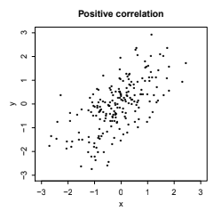
Fig. 6.5 This is Figure 7.9 from [BH19], illustrating RVs \(X\) and \(Y\) which are positively correlated.

A correlation close to 1 indicates a positive linear relationship, as in Fig. 6.5.

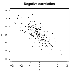
Fig. 6.6 This is Figure 7.9 from [BH19], illustrating RVs \(X\) and \(Y\) which are negatively correlated.

Meanwhile, a correlation close to -1 indicates a negative linear relationship, as in Fig. 6.6.

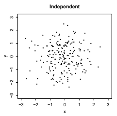
Fig. 6.7 This is Figure 7.9 from [BH19], illustrating RVs \(X\) and \(Y\) which are independent and thus uncorrelated.

Finally, a value closer to 0 suggest a weaker linear relationship, as in Fig. 6.7.

6.4. Multinomial

Before we introduce the next joint distribution, which is a simple generalization of the Binomial distribution, we begin with a quick counting problem.

Counting problem

How many unique ways are there to permute the letters in the word “STATISTICS”?

We start by noting that there are 10 letters in total, but some letters are repeated. Specifically, there are 3 S’s, 3 T’s, 2 I’s, 1 A, and 1 C. To find the number of distinct arrangements, imagine filling in 10 blanks with these letters. First, we choose 3 positions out of 10 for the S’s, which can be done in \(\binom{10}{3}\) ways. Next, we select 3 out of the remaining 7 positions for the T’s, done in \(\binom{7}{3}\) ways, and so on for each letter group.

The total number of distinct permutations is therefore:

\[\begin{equation*} \binom{10}{3} \cdot \binom{7}{3} \cdot \binom{4}{1} \cdot \binom{3}{2} \cdot \binom{1}{1} = \frac{10!}{3!3!2!}. \end{equation*}\]

This result can also be derived by noting that there are \(10!\) ways to arrange all 10 letters if they were distinct, but this count includes overcounting due to the repeated letters. We correct for this by dividing by \(3!\) for the S’s, \(3!\) for the T’s, and \(2!\) for the I’s. Therefore, the total number of distinct arrangements of the letters in “STATISTICS” is given by \(\frac{10!}{3!3!2!}\).

Remember that the Binomial distribution, denoted as Bin\((n, p)\), counts the number of successes in \(n\) trials, where each trial has two possible outcomes: success or failure, with a probability of success \(p\) for each trial.

The Multinomial distribution is a generalization of the Binomial, extending it to scenarios with multiple categories rather than just two. For instance, in a setting where each trial could result in one of three outcomes, such as a win, tie, or loss, the Multinomial distribution is relevant.

Multinomial distribution

Suppose \(n\) objects are placed into \(k\) different categories. Each object has a probability \(p_1\) of being placed in category 1, \(p_2\) in category 2, and so forth, up to category \(k\), where the probabilities sum to 1: \(p_1 + p_2 + \dots + p_k = 1\).

Define \(X_1\) as the number of objects placed in category 1, \(X_2\) as the number in category 2, and so on. The vector \(\vec{X} = (X_1, \dots, X_k)\) follows a Multinomial distribution with parameters \(n\) and \(\vec{p} = (p_1, \dots, p_k)\), denoted as \(\vec{X} \sim \text{Mult}_k(n, \vec{p})\).

To compute the joint PMF, we start with an example. Suppose \(n = 11\) and there are three categories. Then the probability of the specific outcome \(\mathbb{P}[23311112221)]\), which we use to denote the outcome where object 1 is placed in category 2, object 2 is placed in category 3, object 3 is placed in category 3, and so on, is \(\mathbb{P}[23311112221)] = p_1^5p_2^4p_3^2\). This is because there are five 1’s, four 2’s, and two 3’s. As we know from the counting problem at the beginning of this section, there are \(\frac{11!}{5!4!2!}\) ways to construct a sequence with exactly five 1’s, four 2’s, and two 3’s, so

\[\begin{equation*} \mathbb{P}[(X_1 = 5, X_2 = 4, X_3 = 2)] = \frac{11!}{5!4!2!} \cdot p_1^5p_2^4p_3^2. \end{equation*}\]

Generalizing this intuition, we get the joint PMF of the multinomial distribution:

\[\begin{equation*}\mathbb{P}[X_1 = n_1, X_2 = n_2, \dots, X_k = n_k] =\begin{cases} \frac{n!}{n_1!n_2! \dots n_k!}\cdot p_1^{n_1}p_2^{n_2}\cdots p_k^{n_k} &\text{if }n_1 + n_2 + \cdots + n_k = n\\ 0 &\text{else.}\end{cases}\end{equation*}\]

There are a few nice properties of the Multinomial distribution. First, given \(\vec{X} \sim \text{Mult}_k(n, \vec{p})\), where \(\vec{X} = (X_1, X_2, \dots, X_k)\) follows a Multinomial distribution with parameters \(n\) and probability vector \(\vec{p} = (p_1, p_2, \dots, p_k)\), the marginal distribution of each individual component \(X_j\) is Binomial. Specifically, \(X_j \sim \text{Bin}(n, p_j)\), meaning that the count of objects in any single category \(j\) follows a Binomial distribution with probability \(p_j\).

Moreover, the Multinomial distribution also exhibits a property known as the lumping property. This property allows us to combine counts across categories. For example, imagine a political context with five parties, where parties 1 and 2 are dominant, and parties 3, 4, and 5 are minor. We can define a new vector \(\vec{Y} = (X_1, X_2, X_3 + X_4 + X_5)\), where \(X_3 + X_4 + X_5\) represents the combined count of the minor parties. Then \(\vec{Y}\) will follow a Multinomial distribution with three categories and a probability vector adjusted for the combined minor parties: \(\vec{Y} \sim \text{Mult}_3(n, p_1, p_2, p_3 + p_4 + p_5)\).

6.5. Multivariate Normal

Before introducing our final joint distribution, we start with an important property of Normal random variables: if \( Z_1 \sim N(\mu_1, \sigma_1^2) \) and \( Z_2 \sim N(\mu_2, \sigma_2^2) \), then a linear combination of these variables, \( t_1Z_1 + t_2Z_2 \), also follows a Normal distribution. Specifically,

\[\begin{equation*} t_1Z_1 + t_2Z_2 \sim N\left(t_1\mu_1 + t_2\mu_2, t_1^2\sigma_1^2 + t_2^2\sigma_2^2\right). \end{equation*}\]

In many applications, such as finance and data science, it is helpful to work with multidimensional bell curves, which are modeled using the multivariate Normal distribution.

Bivariate normal

The pair \((X, Y)\) has the Bivariate Normal distribution if any linear combination \(aX + bY\) has a Normal distribution for any choice of constants \(a\) and \(b\).

For example, consider \(Z_1 \sim N(\mu_1, \sigma_1^2)\) and \(Z_2 \sim N(\mu_2, \sigma_2^2)\). The pair \((Z_1 - 5Z_2, Z_2)\) is bivariate Normal because any linear combination \(a(Z_1 - 5Z_2) + bZ_2\) simplifies to \(aZ_1 + (5 - b)Z_2\), which, as we know from the useful property at the beginning of this section, is Normally distributed.

A bivariate Normal distribution for \((X, Y)\) is typically denoted as \((X, Y) \sim N(\vec{\mu}, \Sigma)\), where:

• \(\vec{\mu} = (\mathbb{E}[X], \mathbb{E}[Y])\) is the mean vector, and

• \(\Sigma = \begin{pmatrix} \text{Var}(X) & \text{Cov}(X, Y) \\ \text{Cov}(X, Y) & \text{Var}(Y) \end{pmatrix}\) is the covariance matrix, capturing the variances of \(X\) and \(Y\) as well as their covariance.

A noteworthy property of the Bivariate Normal distribution is that if \((X, Y)\) follows this distribution, then both \(X\) and \(Y\) are individually Normally distributed.

One special result for the Bivariate Normal distribution is that if the covariance between \(X\) and \(Y\), \(\text{Cov}(X, Y)\), is zero, then \(X\) and \(Y\) are independent. This property is unique to the Normal distribution, as, in general, zero covariance does not imply independence.