9. Inequalities and limit theorems

9.1. Inequalities

In this section, we’ll cover some tools for back-of-the-envelope estimations of how likely certain events are without knowing the full probability distribution of a random variable. Two fundamental inequalities—Markov’s and Chebyshev’s—are particularly useful for this purpose.

Markov’s inequality

Markov’s inequality states that for any \( a > 0 \), the probability that the absolute value of a random variable \( X \) exceeds \( a \) is bounded by:

\[\begin{equation*} \mathbb{P}[|X| \geq a] \leq \frac{\mathbb{E}[|X|]}{a}. \end{equation*}\]

Example: Ages

Suppose we have a group of 100 people. Let \(X\) be a RV that represents a randomly chosen person’s age.

Question 1: Is it possible for 95 people to be younger than the average age? Yes, for example, we could have 95 infants aged 0 and 5 young adults aged 21. The average age is \(\frac{21}{100}\), and the 95 infants are all younger than this.

Question 2: Can at least 51 people be older than twice the average age? We can answer this question by ordering the ages as \( x_1 \geq x_2 \geq \cdots \geq x_{100} \). By definition,

\[\begin{equation*} \mathbb{E}[X] = \sum_x x \mathbb{P}[X = x] = \frac{1}{100} \sum_{i=1}^{100} x_i = \frac{1}{100} \left( \sum_{i=1}^{51} x_i + \sum_{i=52}^{100} x_i \right). \end{equation*}\]

Assume that at least 51 people are older than twice the average age, so \( x_i \geq 2\mathbb{E}[X] \) for \( i = 1, \dots, 51 \). Substituting this:

\[\begin{equation*} \mathbb{E}[X] \geq \frac{1}{100} \left( \sum_{i=1}^{51} 2\mathbb{E}[X] + \sum_{i=52}^{100} x_i \right) = \frac{1}{100} \left( 102\mathbb{E}[X] + \sum_{i=52}^{100} X_i \right) > \mathbb{E}[X]. \end{equation*}\]

We’ve arrived at a contradiction! Thus, it is not possible for at least 51 people to be older than twice the average age.

We can also answer this question using Markov’s inequality. The fraction of people whose age is at least twice the average is:

\[\begin{equation*} \frac{\text{# people with age } x_i \geq 2\mathbb{E}[X]}{100} = \mathbb{P}[X \geq 2\mathbb{E}[X]] \leq \frac{\mathbb{E}[X]}{2\mathbb{E}[X]} = \frac{1}{2}. \end{equation*}\]

Therefore, at most 50 people can have an age that is at least twice the average.

Chebyshev’s inequality provides a stronger bound by incorporating the variance of the random variable.

Chebyshev’s inequality

Let \( \mu = \mathbb{E}[X] \) and \( \sigma^2 = \text{Var}(X) \). For any \( a > 0 \), Chebyshev’s inequality states:

\[\begin{equation*} \mathbb{P}[|X - \mu| \geq a] \leq \frac{\sigma^2}{a^2}. \end{equation*}\]

This inequality quantifies how spread out the values of \( X \) can be from its mean \( \mu \). For example, it ensures that most of the probability mass is concentrated near the mean when the variance is small.

9.2. Sample mean and variance

Let \( X_1, X_2, \dots, X_n \) represent random variables (RVs) that are identically distributed with an unknown mean \( \mu \) and variance \( \sigma^2 \), i.e.,

\[\begin{equation*} \mathbb{E}[X_1] = \mathbb{E}[X_2] = \cdots = \mathbb{E}[X_n] = \mu \quad \text{and} \quad \text{Var}(X_1) = \text{Var}(X_2) = \cdots = \text{Var}(X_n) = \sigma^2. \end{equation*}\]

We will motivate this section’s key concepts—sample mean and variance—through an example of tracking a stock price’s movement. Suppose \( X_i \) is defined as follows:

\[\begin{equation*} X_i = \begin{cases} 1 & \text{if the stock price increases on day } i, \\ 0 & \text{otherwise.} \end{cases} \end{equation*}\]

Here, \( X_1, X_2, \dots, X_n \) follow a Bernoulli distribution with parameter \( p \), where \( p = \mathbb{P}[X_i = 1] \) represents the probability of a price increase. However, suppose \( p \) is unknown. For instance, if \( n = 5 \) and the observed values are \( X_1 = 1, X_2 = 1, X_3 = 0, X_4 = 1, X_5 = 0 \), the sample mean

\[\begin{equation*} \frac{1}{5}(X_1 + X_2 + X_3 + X_4 + X_5) = \frac{3}{5} \end{equation*}\]

provides a reasonable estimate for \( p \).

Sample mean

The sample mean is defined as

\[\begin{equation*} \bar{X}_n = \frac{1}{n}(X_1 + X_2 + \cdots + X_n). \end{equation*}\]

Its expected value is:

\[\begin{align*} \mathbb{E}[\bar{X}_n] &= \mathbb{E}\left[\frac{1}{n}(X_1 + X_2 + \cdots + X_n)\right]\\ &= \frac{1}{n}\mathbb{E}[X_1 + X_2 + \cdots + X_n]\\ &= \frac{1}{n}(\mathbb{E}[X_1] + \mathbb{E}[X_2] + \cdots + \mathbb{E}[X_n])\\ &= \mu. \end{align*}\]

We call \( \bar{X}_n \) an unbiased estimator of \( \mu \), meaning its expectation equals \( \mu \).

Sample variance

The sample variance is defined as:

\[\begin{equation*} S_n^2 = \frac{1}{n-1} \sum_{j=1}^n (X_j - \bar{X}_n)^2. \end{equation*}\]

Using the earlier example where \( n = 5 \) and \( \bar{X}_n = \frac{3}{5} \), the calculation for \( S_n^2 \) becomes:

\[\begin{equation*} S_n^2 = \frac{1}{4} \left(\left(1 - \frac{3}{5}\right)^2 + \left(1 - \frac{3}{5}\right)^2 + \left(0 - \frac{3}{5}\right)^2 + \left(1 - \frac{3}{5}\right)^2 + \left(0 - \frac{3}{5}\right)^2\right) = \frac{7}{20}. \end{equation*}\]

The sample variance \( S_n^2 \) is a good estimator for the population variance \( \sigma^2 \). Importantly, \( \mathbb{E}[S_n^2] = \sigma^2 \), so \( S_n^2 \) is an unbiased estimator of \( \sigma^2 \).

9.3. Law of Large Numbers

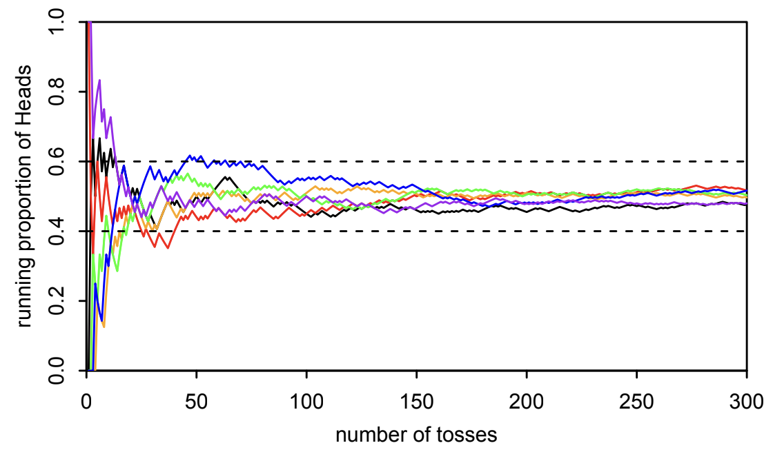
The Law of Large Numbers (LLN) states that as the sample size \( n \) approaches infinity, the sample mean \( \bar{X}_n \) converges to its expected value \(\mathbb{E}\left[ \bar{X}_n\right] = \mu \) with probability 1. In other words, given a sufficiently large number of observations, the average of those observations will almost surely approximate the expected value of the underlying distribution. The LLN is illustrated in Fig. 9.1.

Fig. 9.1 This is Figure 10.2 from [BH19], illustrating the LLN. The figure’s caption in the textbook: “let \( X_1, X_2, \dots \) be i.i.d. \( \text{Bern}\left(\frac{1}{2}\right) \). Interpreting the \( X_j \) as indicators of Heads in a string of fair coin tosses, \( \bar{X}_n \) represents the proportion of Heads after \( n \) tosses. The [LLN] states that, with probability 1, when the sequence of RVs \( \bar{X}_1, \bar{X}_2, \bar{X}_3, \dots \) crystallizes into a sequence of numbers, the sequence of numbers will converge to \(\frac{1}{2}\). Mathematically, there are bizarre outcomes such as \(HHHHHH\dots \) and \(HHTHHTHHTHHT\dots\), but collectively they have zero probability of occurring. […] As an illustration, we simulated six sequences of fair coin tosses” (illustrated by the six different colors in the figure) “and, for each sequence, computed \( \bar{X}_n \) as a function of \( n \). Of course, in real life, we cannot simulate infinitely many coin tosses, so we stopped after 300 tosses. [This figure] plots \( \bar{X}_n \) as a function of \( n \) for each sequence. At the beginning, we can see that there is quite a bit of fluctuation in the running proportion of Heads. As the number of coin tosses increases, however \(\text{Var}(\bar{X}_n)\) gets smaller and smaller, and \(\bar{X}_n\) approaches \(\frac{1}{2}\).”

9.4. Central Limit Theorem

According to the LLN, as \(n \to \infty\), the sample mean \(\bar{X}_n\) converges to the constant value \(\mathbb{E}\left[ \bar{X}_n\right]\), but as we can see from Fig. 9.1, for intermediate values of \(n\), \(\bar{X}_n\) still exhibits random behavior. This raises the question: what is the distribution of \(\bar{X}_n\)? This question is answered by the central limit theorem (CLT), a cornerstone of probability and statistics.

Central limit theorem

Let \( X_1, X_2, \dots, X_n \) be random variables drawn from the same arbitrary distribution with expected value \(\mu\) and variance \(\sigma^2\):

\[\begin{equation*} \mathbb{E}[X_1] = \mathbb{E}[X_2] = \cdots = \mathbb{E}[X_n] = \mu, \quad \text{and} \quad \text{Var}(X_1) = \text{Var}(X_2) = \cdots = \text{Var}(X_n) = \sigma^2. \end{equation*}\]

Even if the underlying distribution of \( X_1, \dots, X_n \) is not normal, the central limit theorem guarantees that, for large \( n \), the distribution of the sample mean:

\[\begin{equation*} \bar{X}_n = \frac{1}{n} \sum_{i=1}^n X_i \end{equation*}\]

is approximately normal. Specifically, \( \bar{X}_n \) is approximately distributed as:

\[\begin{equation*} \mathcal{N}\left(\mu, \frac{\sigma^2}{n}\right). \end{equation*}\]

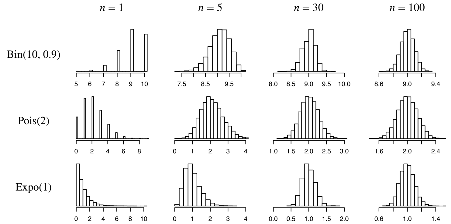
The central limit theorem is illustrated in Fig. 9.2.

Fig. 9.2 This is Figure 10.5 from [BH19], illustrating the central limit theorem. The figure’s caption in the textbook: “Histograms of the distribution of \(\bar{X}_n\) for different starting distributions of the \(X_j\) (indicated by the rows) and increasing values of \(n\) (indicated by the columns). Each histogram is based on 10,000 simulated values of \(\bar{X}_n\). Regardless of the starting distribution of the \(X_j\), the distribution of \(\bar{X}_n\) approaches a Normal distribution as \(n\) grows.”

Example: Bernoulli

Suppose \( X_1, \dots, X_n \sim \text{Bern}(p) \) with \( p = \frac{1}{2} \). For each \( X \), we have:

\[\begin{equation*} \mathbb{E}[X] = p = \frac{1}{2}, \quad \text{Var}(X) = p(1-p) = \frac{1}{4}. \end{equation*}\]

Now, define the sample mean:

\[\begin{equation*} \bar{X}_n = \frac{1}{n}(X_1 + \cdots + X_n). \end{equation*}\]

By the Central Limit Theorem, when \( n \) is large, \( \bar{X}_n \) is approximately distributed as:

\[\begin{equation*} \mathcal{N}\left(\frac{1}{2}, \frac{1}{4n}\right). \end{equation*}\]

Example: Binomial

This is Example 10.3.3 from [BH19].

Let \( Y \sim \text{Bin}\left(n, \frac{1}{2}\right) \), where \( n \) is large. The binomial random variable \( Y \) can be expressed as the sum of independent Bernoulli random variables:

\[\begin{equation*} Y = X_1 + \cdots + X_n, \quad \text{where } X_1, \dots, X_n \sim \text{Bern}\left(\frac{1}{2}\right). \end{equation*}\]

Using the relationship \( Y = n\bar{X}_n \), the normalized variable \( \bar{X}_n = \frac{1}{n} Y \) is approximately distributed as:

\[\begin{equation*} \mathcal{N}\left(\frac{1}{2}, \frac{1}{4n}\right). \end{equation*}\]

Consequently, \( Y \) itself is approximately distributed as:

\[\begin{equation*} \mathcal{N}\left(\frac{n}{2}, \frac{n}{4}\right). \end{equation*}\]

Example: Log-normal

This is Example 10.3.7 from [BH19].

In Section 7.1, I claimed that if \(X \sim N(0,1)\) is normally distributed, then \(Y = e^X\) is often used to model the evolution of stock prices. In this example, we will see why this is!

Suppose a stock price either rises by 70% or falls by 50% each day, with both outcomes equally likely. Let \( Y_n \) denote the stock price after \( n = 365 \) days, starting with an initial price \( Y_0 = 100 \). The goal is to use the Central Limit Theorem (CLT) to demonstrate that \( \log Y_n \) is approximately normally distributed. Specifically, this means that \( Y_n \) can be expressed as \( Y_n \approx e^X \), where \( X \) is drawn from a normal distribution.

Let \( U_n \) denote the number of days the stock price rises within the first \( n \) days. Consequently, \( n - U_n \) represents the number of days the stock price falls. The stock price after the first day, \( Y_1 \), is given by:

\[\begin{equation*} Y_1 = \begin{cases} Y_0 \cdot 1.7 & \text{if the stock rises on day 1 (i.e., $ U_1 = 1 $)}, \\ Y_0 \cdot 0.5 & \text{if the stock falls on day 1 (i.e., $ U_1 = 0 $)}. \end{cases} \end{equation*}\]

This can be rewritten as:

\[\begin{equation*} Y_1 = Y_0 \cdot (1.7)^{U_1} \cdot (0.5)^{1 - U_1}. \end{equation*}\]

By generalizing this to \( n \) days, the stock price after \( n \) days becomes:

\[\begin{equation*} Y_n = Y_0 \cdot (1.7)^{U_n} \cdot (0.5)^{n - U_n}. \end{equation*}\]

Taking the logarithm of \( Y_n \), we use the properties of logarithms (\( \log(ab) = \log a + \log b \) and \( \log(a^b) = b \log a \)) to write:

\[\begin{equation*} \log Y_n = \log Y_0 + U_n \log 1.7 + (n - U_n) \log 0.5. \end{equation*}\]

Combining terms involving \( U_n \):

\[\begin{equation*} \log Y_n = \log Y_0 + U_n \log 3.4 + n \log 0.5. \end{equation*}\]

Letting \(C = \log Y_0 + n \log 0.5 \) represent a constant (i.e., it is not random), we can write this as:

\[\begin{equation*} \log Y_n = U_n \log 3.4 + C. \end{equation*}\]

The random variable \( U_n \), which counts the number of days the stock rises, follows a binomial distribution:

\[\begin{equation*} U_n \sim \text{Bin}\left(n, \frac{1}{2}\right). \end{equation*}\]

For large \( n \), the Central Limit Theorem guarantees that \( U_n \) can be approximated by a normal distribution:

\[\begin{equation*} U_n \sim \mathcal{N}\left(\frac{n}{2}, \frac{n}{4}\right). \end{equation*}\]

Since \( \log Y_n \) is a linear transformation of \( U_n \), and a linear transformation of a normally distributed random variable remains normal, we conclude that \( \log Y_n \) is approximately normally distributed.